深度学习-9-pytorch-1-基本概念

本文最后更新于:2021年8月10日 晚上

创作声明:主要内容参考于张贤同学https://zhuanlan.zhihu.com/p/265394674

前言

在使用pytorch进行深度学习训练时,我们需要有一个规范的步骤流程。这个流程可以让构建自己的代码和阅读别人的代码时思路清晰,心中有底。

步骤思想

  1. 数据处理(包括数据读取,数据清洗,进行数据划分和数据预处理,比如读取图片如何预处理及数据增强,使数据变成网络能够处理的tensor类型,输入数据)
  2. 模型构建(包括构建模型模块,组织复杂网络,初始化网络参数,定义网络层)
  3. 损失函数(包括创建损失函数,设置损失函数超参数,根据不同任务选择合适的损失函数)
  4. 优化器(包括根据梯度使用某种优化器更新参数,管理模型参数,管理多个参数组实现不同学习率,调整学习率。)
  5. 迭代训练(组织上面 4 个模块进行反复训练。还包括观察训练效果,绘制 Loss/ Accuracy 曲线,用 TensorBoard 进行可视化分析)

    Tensor 操作

    概念

    Tensor 中文为张量。张量的意思是一个多维数组,它是标量、向量、矩阵的高维扩展。

标量可以称为 0 维张量,向量可以称为 1 维张量,矩阵可以称为 2 维张量,RGB 图像可以表示 3 维张量。你可以把张量看作多维数组。

Tensor的属性:

  • data: 被包装的 Tensor。
  • grad: data 的梯度。
  • grad_fn: 创建 Tensor 所使用的 Function,是自动求导的关键,因为根据所记录的函数才能计算出导数。
  • requires_grad: 指示是否需要梯度,并不是所有的张量都需要计算梯度。
  • is_leaf: 指示张量是否叶子节点,叶子节点的概念在计算图中会用到,后面详细介绍。
  • dtype: 张量的数据类型,如 torch.FloatTensor,torch.cuda.FloatTensor。
  • shape: 张量的形状。如 (64, 3, 224, 224)
  • device: 张量所在设备 (CPU/GPU),GPU 是加速计算的关键。

    创建Tensor

    直接创建

  1. torch.tensor()
    1
    torch.tensor(data, dtype=None, device=None, requires_grad=False, pin_memory=False)
  • data: 数据,可以是 list,numpy
  • dtype: 数据类型,默认与 data 的一致
  • device: 所在设备,cuda/cpu
  • requires_grad: 是否需要梯度
  • pin_memory: 是否存于锁页内存

代码示例:

1
2
3
4
5
6
arr = np.ones((3, 3))
print("ndarray的数据类型:", arr.dtype)
# 创建存放在 GPU 的数据
# t = torch.tensor(arr, device='cuda')
t= torch.tensor(arr)
print(t)

输出为:

1
2
3
4
ndarray的数据类型: float64
tensor([[1., 1., 1.],
[1., 1., 1.],
[1., 1., 1.]], dtype=torch.float64)
  1. torch.from_numpy(ndarray)
    从 numpy 创建 tensor。利用这个方法创建的 tensor 和原来的 ndarray 共享内存,当修改其中一个数据,另外一个也会被改动。

代码示例:

1
2
3
4
5
6
7
8
9
10
11
12
13
14
arr = np.array([[1, 2, 3], [4, 5, 6]])
t = torch.from_numpy(arr)

# 修改 array,tensor 也会被修改
# print("\n修改arr")
# arr[0, 0] = 0
# print("numpy array: ", arr)
# print("tensor : ", t)

# 修改 tensor,array 也会被修改
print("\n修改tensor")
t[0, 0] = -1
print("numpy array: ", arr)
print("tensor : ", t)

输出为:

1
2
3
4
5
修改tensor
numpy array: [[-1 2 3]
[ 4 5 6]]
tensor : tensor([[-1, 2, 3],
[ 4, 5, 6]], dtype=torch.int32)

根据数值创建 Tensor

  1. torch.zeros()
    1
    torch.zeros(*size, out=None, dtype=None, layout=torch.strided, device=None, requires_grad=False)
    功能:根据 size 创建全 0 张量
  • size: 张量的形状
  • out: 输出的张量,如果指定了 out,那么将新建的zero张量写入到out张量中,不指定out则新建一个张量,然后无论如何,返回表示这个新的全0矩阵的张量。
  • layout: 内存中布局形式,有 strided,sparse_coo 等。当是稀疏矩阵时,设置为 sparse_coo 可以减少内存占用。
  • device: 所在设备,cuda/cpu
  • requires_grad: 是否需要梯度

代码示例:

1
2
3
4
5
6
out_t = torch.tensor([1])
# 这里制定了 out
t = torch.zeros((3, 3), out=out_t)
print(t, '\n', out_t)
# id 是取内存地址。最终 t 和 out_t 是同一个内存地址
print(id(t), id(out_t), id(t) == id(out_t))

输出是:

1
2
3
4
5
6
7
tensor([[0, 0, 0],
[0, 0, 0],
[0, 0, 0]])
tensor([[0, 0, 0],
[0, 0, 0],
[0, 0, 0]])
2984903203072 2984903203072 True
  1. torch.zeros_like
    1
    torch.zeros_like(input, dtype=None, layout=None, device=None, requires_grad=False, memory_format=torch.preserve_format)
    功能:根据 input 形状创建全 0 张量
  • input: 创建与 input 同形状的全 0 张量
  • dtype: 数据类型
  • layout: 内存中布局形式,有 strided,sparse_coo 等。当是稀疏矩阵时,设置为 sparse_coo 可以减少内存占用。

同理还有全 1 张量的创建方法:torch.ones(),torch.ones_like()。

  1. torch.full(),torch.full_like()
    1
    torch.full(size, fill_value, out=None, dtype=None, layout=torch.strided, device=None, requires_grad=False)
    功能:创建自定义数值的张量
  • size: 张量的形状,如 (3,3)
  • fill_value: 张量中每一个元素的值

代码示例:

1
2
t = torch.full((3, 3), 1)
print(t)

输出为:

1
2
3
tensor([[1., 1., 1.],
[1., 1., 1.],
[1., 1., 1.]])
  1. torch.arange()
    1
    torch.arange(start=0, end, step=1, out=None, dtype=None, layout=torch.strided, device=None, requires_grad=False)
    功能:创建等差的 1 维张量。注意区间为[start, end)。
  • start: 数列起始值
  • end: 数列结束值,开区间,取不到结束值
  • step: 数列公差,默认为 1

代码示例:

1
2
t = torch.arange(2, 10, 2)
print(t)

输出为:

1
tensor([2, 4, 6, 8])
  1. torch.linspace()
    1
    torch.linspace(start, end, steps=100, out=None, dtype=None, layout=torch.strided, device=None, requires_grad=False)
    功能:创建均分的 1 维张量。数值区间为 [start, end]
  • start: 数列起始值
  • end: 数列结束值
  • steps: 数列长度 (元素个数)

代码示例:

1
2
3
# t = torch.linspace(2, 10, 5)
t = torch.linspace(2, 10, 6)
print(t)

输出为:

1
tensor([ 2.0000,  3.6000,  5.2000,  6.8000,  8.4000, 10.0000])
  1. torch.logspace()
    1
    torch.logspace(start, end, steps=100, base=10.0, out=None, dtype=None, layout=torch.strided, device=None, requires_grad=False)
    功能:创建对数均分的 1 维张量。数值区间为 [start, end],底为 base。
  • start: 数列起始值
  • end: 数列结束值
  • steps: 数列长度 (元素个数)
  • base: 对数函数的底,默认为 10

代码示例:

1
2
3
# t = torch.logspace(2, 10, 5)
t = torch.logspace(2, 10, 6)
print(t)

输出为:

1
tensor([ 2.0000,  3.6000,  5.2000,  6.8000,  8.4000, 10.0000])
  1. torch.eye()
    1
    torch.eye(n, m=None, out=None, dtype=None, layout=torch.strided, device=None, requires_grad=False)
    功能:创建单位对角矩阵( 2 维张量),默认为方阵
  • vn: 矩阵行数。通常只设置 n,为方阵。
  • m: 矩阵列数

    根据概率创建 Tensor

  1. torch.normal()
    1
    torch.normal(mean, std, *, generator=None, out=None)
    功能:生成正态分布 (高斯分布)
  • mean: 均值
  • std: 标准差

有 4 种模式:

  • mean 为标量,std 为标量。

代码示例:

1
2
3
# mean:标量 std: 标量 这里需要设置 size 
t_normal = torch.normal(0., 1., size=(4,))
print(t_normal)

输出为:

1
tensor([0.6614, 0.2669, 0.0617, 0.6213])
  • mean 为标量,std 为张量
  • mean 为张量,std 为标量

代码示例:

1
2
3
4
5
6
# mean:张量 std: 标量
mean = torch.arange(1, 5, dtype=torch.float)
std = 1
t_normal = torch.normal(mean, std)
print("mean:{}\nstd:{}".format(mean, std))
print(t_normal)

输出为:

1
2
3
mean:tensor([1., 2., 3., 4.])
std:1
tensor([1.6614, 2.2669, 3.0617, 4.6213])

这 4 个数采样分布的均值不同,但是方差都是 1。

  • mean 为张量,std 为张量

代码示例:

1
2
3
4
5
6
# mean:张量 std: 张量
mean = torch.arange(1, 5, dtype=torch.float)
std = torch.arange(1, 5, dtype=torch.float)
t_normal = torch.normal(mean, std)
print("mean:{}\nstd:{}".format(mean, std))
print(t_normal)

输出为:

1
2
3
mean:tensor([1., 2., 3., 4.])
std:tensor([1., 2., 3., 4.])
tensor([1.6614, 2.5338, 3.1850, 6.4853])

其中 1.6614 是从正态分布$N(1,1)$ 中采样得到的,其他数字以此类推。

  1. torch.randn() 和 torch.randn_like()
    1
    torch.randn(*size, out=None, dtype=None, layout=torch.strided, device=None, requires_grad=False)
    功能:生成标准正态分布。
  • size: 张量的形状
  1. torch.rand() 和 torch.rand_like()
    1
    torch.rand(*size, out=None, dtype=None, layout=torch.strided, device=None, requires_grad=False)
    功能:在区间 [0, 1) 上生成均匀分布。
  2. torch.randint() 和 torch.randint_like()
    1
    2
    randint(low=0, high, size, *, generator=None, out=None,
    dtype=None, layout=torch.strided, device=None, requires_grad=False)
    功能:在区间 [low, high) 上生成整数均匀分布。
  • n: 张量的形状
  1. torch.randperm()
    1
    torch.randperm(n, out=None, dtype=torch.int64, layout=torch.strided, device=None, requires_grad=False)
    功能:生成从 0 到 n-1 的随机排列。常用于生成索引。
  • n: 张量的长度
  1. torch.bernoulli()
    1
    torch.bernoulli(input, *, generator=None, out=None)
    功能:以 input 为概率,生成伯努利分布 (0-1 分布,两点分布)
  • input: 概率值

    拼接切分Tensor

  1. torch.cat()
    1
    torch.cat(tensors, dim=0, out=None)
    功能:将张量按照 dim 维度进行拼接
  • tensors: 张量序列
  • dim: 要拼接的维度

代码示例:

1
2
3
4
t = torch.ones((2, 3))
t_0 = torch.cat([t, t], dim=0)
t_1 = torch.cat([t, t], dim=1)
print("t_0:{} shape:{}\nt_1:{} shape:{}".format(t_0, t_0.shape, t_1, t_1.shape))

输出:

1
2
3
4
5
6
t_0:tensor([[1., 1., 1.],
[1., 1., 1.],
[1., 1., 1.],
[1., 1., 1.]]) shape:torch.Size([4, 3])
t_1:tensor([[1., 1., 1., 1., 1., 1.],
[1., 1., 1., 1., 1., 1.]]) shape:torch.Size([2, 6])
  1. torch.stack()
    1
    torch.stack(tensors, dim=0, out=None)
    功能:将张量在新创建的 dim 维度上进行拼接
  • tensors: 张量序列
  • dim: 要拼接的维度

代码示例:

1
2
3
4
5
6
7
t = torch.ones((2, 3))
# dim =2
t_stack = torch.stack([t, t, t], dim=2)
print("\nt_stack.shape:{}".format(t_stack.shape))
# dim =0
t_stack = torch.stack([t, t, t], dim=0)
print("\nt_stack.shape:{}".format(t_stack.shape))

输出为:

1
2
t_stack.shape:torch.Size([2, 3, 3])
t_stack.shape:torch.Size([3, 2, 3])

第一次指定拼接的维度 dim =2,结果的维度是 [2, 3, 3]。后面指定拼接的维度 dim =0,由于原来的 tensor 已经有了维度 0,因此会把 tensor 往后移动一个维度变为 [1,2,3],再拼接变为 [3,2,3]。
3. torch.chunk()

1
torch.chunk(input, chunks, dim=0)

功能:将张量按照维度 dim 进行平均切分。若不能整除,则最后一份张量小于其他张量。

  • input: 要切分的张量
  • chunks: 要切分的份数
  • dim: 要切分的维度

代码示例:

1
2
3
4
a = torch.ones((2, 7))  # 7
list_of_tensors = torch.chunk(a, dim=1, chunks=3) # 3
for idx, t in enumerate(list_of_tensors):
print("第{}个张量:{}, shape is {}".format(idx+1, t, t.shape))

输出为:

1
2
3
4
5
6
第1个张量:tensor([[1., 1., 1.],
[1., 1., 1.]]), shape is torch.Size([2, 3])
第2个张量:tensor([[1., 1., 1.],
[1., 1., 1.]]), shape is torch.Size([2, 3])
第3个张量:tensor([[1.],
[1.]]), shape is torch.Size([2, 1])

由于 7 不能整除 3,7/3 再向上取整是 3,因此前两个维度是 [2, 3],所以最后一个切分的张量维度是 [2,1]。
4. torch.split()

1
torch.split(tensor, split_size_or_sections, dim=0)

功能:将张量按照维度 dim 进行平均切分。可以指定每一个分量的切分长度。

  • tensor: 要切分的张量
  • split_size_or_sections: 为 int 时,表示每一份的长度,如果不能被整除,则最后一份张量小于其他张量;为 list 时,按照 list 元素作为每一个分量的长度切分。如果 list 元素之和不等于切分维度 (dim) 的值,就会报错。
  • dim: 要切分的维度

代码示例:

1
2
3
4
t = torch.ones((2, 5))
list_of_tensors = torch.split(t, [2, 1, 2], dim=1)
for idx, t in enumerate(list_of_tensors):
print("第{}个张量:{}, shape is {}".format(idx+1, t, t.shape))

结果为:

1
2
3
4
5
6
第1个张量:tensor([[1., 1.],
[1., 1.]]), shape is torch.Size([2, 2])
第2个张量:tensor([[1.],
[1.]]), shape is torch.Size([2, 1])
第3个张量:tensor([[1., 1.],
[1., 1.]]), shape is torch.Size([2, 2])

Tensor 索引

  1. torch.index_select()
    1
    torch.index_select(input, dim, index, out=None)
    功能:在维度 dim 上,按照 index 索引取出数据拼接为张量返回。
  • input: 要索引的张量
  • dim: 要索引的维度
  • index: 要索引数据的序号

代码示例:

1
2
3
4
5
6
7
# 创建均匀分布
t = torch.randint(0, 9, size=(3, 3))
# 注意 idx 的 dtype 不能指定为 torch.float
idx = torch.tensor([0, 2], dtype=torch.long)
# 取出第 0 行和第 2 行
t_select = torch.index_select(t, dim=0, index=idx)
print("t:\n{}\nt_select:\n{}".format(t, t_select))

输出为:

1
2
3
4
5
6
7
t:
tensor([[4, 5, 0],
[5, 7, 1],
[2, 5, 8]])
t_select:
tensor([[4, 5, 0],
[2, 5, 8]])
  1. torch.mask_select()
    1
    torch.masked_select(input, mask, out=None)
    功能:按照 mask 中的 True 进行索引拼接得到一维张量返回。
  • input:要索引的张量
  • mask: 与 input 同形状的布尔类型张量

代码示例:

1
2
3
4
5
t = torch.randint(0, 9, size=(3, 3))
mask = t.le(5) # ge is mean greater than or equal/ gt: greater than le lt
# 取出大于 5 的数
t_select = torch.masked_select(t, mask)
print("t:\n{}\nmask:\n{}\nt_select:\n{} ".format(t, mask, t_select))

结果为:

1
2
3
4
5
6
7
8
9
10
t:
tensor([[4, 5, 0],
[5, 7, 1],
[2, 5, 8]])
mask:
tensor([[ True, True, True],
[ True, False, True],
[ True, True, False]])
t_select:
tensor([4, 5, 0, 5, 1, 2, 5])

最后返回的是一维张量。

Tensor 变换

  1. torch.reshape()
    1
    torch.reshape(input, shape)
    功能:变换张量的形状。当张量在内存中是连续时,返回的张量和原来的张量共享数据内存,改变一个变量时,另一个变量也会被改变。
  • input: 要变换的张量
  • shape: 新张量的形状

代码示例:

1
2
3
4
5
# 生成 0 到 8 的随机排列
t = torch.randperm(8)
# -1 表示这个维度是根据其他维度计算得出的
t_reshape = torch.reshape(t, (-1, 2, 2))
print("t:{}\nt_reshape:\n{}".format(t, t_reshape))

结果为:

1
2
3
4
5
6
7
t:tensor([5, 4, 2, 6, 7, 3, 1, 0])
t_reshape:
tensor([[[5, 4],
[2, 6]],

[[7, 3],
[1, 0]]])

在上面代码的基础上,修改原来的张量的一个元素,新张量也会被改变。

代码示例:

1
2
3
4
5
# 修改张量 t 的第 0 个元素,张量 t_reshape 也会被改变
t[0] = 1024
print("t:{}\nt_reshape:\n{}".format(t, t_reshape))
print("t.data 内存地址:{}".format(id(t.data)))
print("t_reshape.data 内存地址:{}".format(id(t_reshape.data)))

结果为:

1
2
3
4
5
6
7
8
9
t:tensor([1024,    4,    2,    6,    7,    3,    1,    0])
t_reshape:
tensor([[[1024, 4],
[ 2, 6]],

[[ 7, 3],
[ 1, 0]]])
t.data 内存地址:2636803119936
t_reshape.data 内存地址:2636803119792
  1. torch.transpose()
    1
    torch.transpose(input, dim0, dim1)
    功能:交换张量的两个维度。常用于图像的变换,比如把chw变换为hwc。
  • input: 要交换的变量
  • dim0: 要交换的第一个维度
  • dim1: 要交换的第二个维度
    代码示例:
    1
    2
    3
    4
    #把 c * h * w 变换为 h * w * c
    t = torch.rand((2, 3, 4))
    t_transpose = torch.transpose(t, dim0=1, dim1=2) # c*h*w h*w*c
    print("t shape:{}\nt_transpose shape: {}".format(t.shape, t_transpose.shape))
    结果为:
    1
    2
    3
    t shape:torch.Size([2, 3, 4])
    t_transpose shape: torch.Size([2, 4, 3])
    torch.t()
    功能:2 维张量转置,对于 2 维矩阵而言,等价于torch.transpose(input, 0, 1)。
  1. torch.squeeze()
    1
    torch.squeeze(input, dim=None, out=None)
    功能:压缩长度为 1 的维度。
  • dim: 若为 None,则移除所有长度为 1 的维度;若指定维度,则当且仅当该维度长度为 1 时可以移除。

代码示例:

1
2
3
4
5
6
7
8
9
10
11
12
# 维度 0 和 3 的长度是 1
t = torch.rand((1, 2, 3, 1))
# 可以移除维度 0 和 3
t_sq = torch.squeeze(t)
# 可以移除维度 0
t_0 = torch.squeeze(t, dim=0)
# 不能移除 1
t_1 = torch.squeeze(t, dim=1)
print("t.shape: {}".format(t.shape))
print("t_sq.shape: {}".format(t_sq.shape))
print("t_0.shape: {}".format(t_0.shape))
print("t_1.shape: {}".format(t_1.shape))

结果为:

1
2
3
4
t.shape: torch.Size([1, 2, 3, 1])
t_sq.shape: torch.Size([2, 3])
t_0.shape: torch.Size([2, 3, 1])
t_1.shape: torch.Size([1, 2, 3, 1])
  1. torch.unsqueeze()
    1
    torch.unsqueeze(input, dim)
    功能:根据 dim 扩展维度,长度为 1。

    Tensor 数学运算

    主要分为 3 类:加减乘除,对数,指数,幂函数 和三角函数。

这里介绍一下常用的几种方法。

  1. torch.add()
    1
    2
    torch.add(input, other, out=None)
    torch.add(input, other, *, alpha=1, out=None)
    功能:逐元素计算 input + alpha * other。因为在深度学习中经常用到先乘后加的操作。
  • input: 第一个张量
  • alpha: 乘项因子
  • other: 第二个张量
  1. torch.addcdiv()
    1
    torch.addcdiv(input, tensor1, tensor2, *, value=1, out=None)
    计算公式为:$out_i = input_i+value\times {tensor1_i\over tensor2_i}$
  2. torch.addcmul()
    1
    torch.addcmul(input, tensor1, tensor2, *, value=1, out=None)
    计算公式为:$out_i = input_i+value\times tensor1_i\times tensor2_i$

    线性回归

    线性回归是分析一个变量 ($y$) 与另外一 (多) 个变量 ($x$) 之间的关系的方法。一般可以写成 $y=wx+b$。线性回归的目的就是求解参数$w,b$。

线性回归的求解可以分为 3 步:

  1. 确定模型:$y=wx+b$
  2. 选择损失函数,一般使用均方误差 MSE:${1\over m} \sum_{i=1}^m(y_i-\hat{y_i})^2$。其中$\hat{y_i}$是预测值,$y$是真实值。
  3. 使用梯度下降法求解梯度 (其中$lr$是学习率),并更新参数:
  • $w=w-lr*w.grad$
  • $b=b-lr*b.grad$

代码如下:

1
2
3
4
5
6
7
8
9
10
11
12
13
14
15
16
17
18
19
20
21
22
23
24
25
26
27
28
29
30
31
32
33
34
35
36
37
38
39
40
41
42
43
44
45
46
47
48
49
50
import torch
import matplotlib.pyplot as plt
torch.manual_seed(10)

lr = 0.05 # 学习率

# 创建训练数据
x = torch.rand(20, 1) * 10 # x data (tensor), shape=(20, 1)
# torch.randn(20, 1) 用于添加噪声
y = 2*x + (5 + torch.randn(20, 1)) # y data (tensor), shape=(20, 1)

# 构建线性回归参数
w = torch.randn((1), requires_grad=True) # 设置梯度求解为 true
b = torch.zeros((1), requires_grad=True) # 设置梯度求解为 true

# 迭代训练 1000 次
for iteration in range(1000):

# 前向传播,计算预测值
wx = torch.mul(w, x)
y_pred = torch.add(wx, b)

# 计算 MSE loss
loss = (0.5 * (y - y_pred) ** 2).mean()

# 反向传播
loss.backward()

# 更新参数
b.data.sub_(lr * b.grad)
w.data.sub_(lr * w.grad)

# 每次更新参数之后,都要清零张量的梯度
w.grad.zero_()
b.grad.zero_()

# 绘图,每隔 20 次重新绘制直线
if iteration % 20 == 0:

plt.scatter(x.data.numpy(), y.data.numpy())
plt.plot(x.data.numpy(), y_pred.data.numpy(), 'r-', lw=5)
plt.text(2, 20, 'Loss=%.4f' % loss.data.numpy(), fontdict={'size': 20, 'color': 'red'})
plt.xlim(1.5, 10)
plt.ylim(8, 28)
plt.title("Iteration: {}\nw: {} b: {}".format(iteration, w.data.numpy(), b.data.numpy()))
plt.pause(0.5)

# 如果 MSE 小于 1,则停止训练
if loss.data.numpy() < 1:
break

训练的直线的可视化如下:

在 80 次的时候,Loss 已经小于 1 了,因此停止了训练。

静态图与动态图机制

计算图

深度学习就是对张量进行一系列的操作,随着操作种类和数量的增多,会出现各种值得思考的问题。比如多个操作之间是否可以并行,如何协同底层的不同设备,如何避免冗余的操作,以实现最高效的计算效率,同时避免一些 bug。因此产生了计算图 (Computational Graph)。

计算图是用来描述运算的有向无环图,有两个主要元素:节点 (Node) 和边 (Edge)。节点表示数据,如向量、矩阵、张量。边表示运算,如加减乘除卷积等。

用计算图表示:$y=(x+w)*(w+1)$,如下所示:

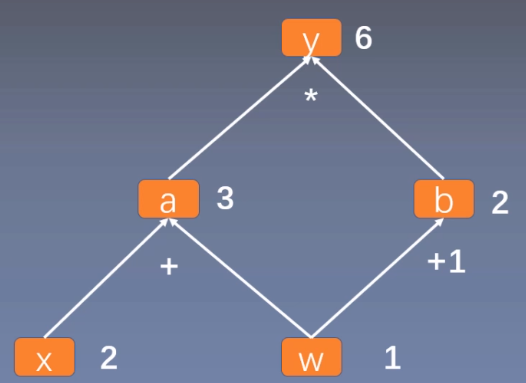
可以看作, $y=a \times b$ ,其中 $a=x+w$,$b=w+1$。

计算图与梯度求导

这里求 $y$ 对 $w$ 的导数。根复合函数的求导法则,可以得到如下过程。
$\begin{aligned} \frac{\partial y}{\partial w} &=\frac{\partial y}{\partial a} \frac{\partial a}{\partial w}+\frac{\partial y}{\partial b} \frac{\partial b}{\partial w} \ &=b 1+a 1 \ &=b+a \ &=(w+1)+(x+w) \ &=2 w+x+1 \ &=2 1+2+1=5\end{aligned}$
体现到计算图中,就是根节点 $y$ 到叶子节点 $w$ 有两条路径 y -> a -> w和y ->b -> w。根节点依次对每条路径的孩子节点求导,一直到叶子节点w,最后把每条路径的导数相加即可。

代码如下:

1
2
3
4
5
6
7
8
9
10
11
import torch
w = torch.tensor([1.], requires_grad=True)
x = torch.tensor([2.], requires_grad=True)
# y=(x+w)*(w+1)
a = torch.add(w, x) # retain_grad()
b = torch.add(w, 1)
y = torch.mul(a, b)
# y 求导
y.backward()
# 打印 w 的梯度,就是 y 对 w 的导数
print(w.grad)

结果为tensor([5.])。

我们回顾前面说过的 Tensor 中有一个属性is_leaf标记是否为叶子节点。
在上面的例子中,$x$ 和 $w$ 是叶子节点,其他所有节点都依赖于叶子节点。叶子节点的概念主要是为了节省内存,在计算图中的一轮反向传播结束之后,非叶子节点的梯度是会被释放的。

代码示例(接上文):

1
2
3
4
5
# 查看叶子结点
print("is_leaf:\n", w.is_leaf, x.is_leaf, a.is_leaf, b.is_leaf, y.is_leaf)

# 查看梯度
print("gradient:\n", w.grad, x.grad, a.grad, b.grad, y.grad)

结果为:

1
2
3
4
is_leaf:
True True False False False
gradient:
tensor([5.]) tensor([2.]) None None None

非叶子节点的梯度为空,如果在反向传播结束之后仍然需要保留非叶子节点的梯度,可以对节点使用retain_grad()方法。

而 Tensor 中的 grad_fn 属性记录的是创建该张量时所用的方法 (函数)。而在反向传播求导梯度时需要用到该属性。

示例代码:

1
2
3
4
5
6
# 查看梯度
print("w.grad_fn = ", w.grad_fn)
print("x.grad_fn = ", x.grad_fn)
print("a.grad_fn = ", a.grad_fn)
print("b.grad_fn = ", b.grad_fn)
print("y.grad_fn = ", y.grad_fn)

结果为

1
2
3
4
5
w.grad_fn =  None
x.grad_fn = None
a.grad_fn = <AddBackward0 object at 0x000001D8DDD20588>
b.grad_fn = <AddBackward0 object at 0x000001D8DDD20588>
y.grad_fn = <MulBackward0 object at 0x000001D8DDD20588>

PyTorch 的动态图机制

PyTorch 采用的是动态图机制 (Dynamic Computational Graph),而 Tensorflow 采用的是静态图机制 (Static Computational Graph)。

动态图是运算和搭建同时进行,也就是可以先计算前面的节点的值,再根据这些值搭建后面的计算图。优点是灵活,易调节,易调试。PyTorch 里的很多写法跟其他 Python 库的代码的使用方法是完全一致的,没有任何额外的学习成本。

静态图是先搭建图,然后再输入数据进行运算。优点是高效,因为静态计算是通过先定义后运行的方式,之后再次运行的时候就不再需要重新构建计算图,所以速度会比动态图更快。但是不灵活。TensorFlow 每次运行的时候图都是一样的,是不能够改变的,所以不能直接使用 Python 的 while 循环语句,需要使用辅助函数 tf.while_loop 写成 TensorFlow 内部的形式。

autograd

自动求导 (autograd)

在深度学习中,权值的更新是依赖于梯度的计算,因此梯度的计算是至关重要的。在 PyTorch 中,只需要搭建好前向计算图,然后利用torch.autograd自动求导得到所有张量的梯度。

torch.autograd.backward()(一次求出所有参数的导数)

1
torch.autograd.backward(tensors, grad_tensors=None, retain_graph=None, create_graph=False, grad_variables=None)

功能:自动求取梯度

  • tensors: 用于求导的张量,如 loss
  • retain_graph: 保存计算图。PyTorch 采用动态图机制,默认每次反向传播之后都会释放计算图。这里设置为 True 可以不释放计算图。
  • create_graph: 创建导数计算图,用于高阶求导
  • grad_tensors: 多梯度权重。当有多个 loss 混合需要计算梯度时,设置每个 loss 的权重。

代码示例:

1
2
3
4
5
6
7
8
9
10
11
12
w = torch.tensor([1.], requires_grad=True)
x = torch.tensor([2.], requires_grad=True)
# y=(x+w)*(w+1)
a = torch.add(w, x)
b = torch.add(w, 1)
y = torch.mul(a, b)

# 第一次执行梯度求导
y.backward()
print(w.grad)
# 第二次执行梯度求导,出错
y.backward()

其中y.backward()方法调用的是torch.autograd.backward(self, gradient, retain_graph, create_graph)。但是在第二次执行y.backward()时会出错。因为 PyTorch 默认是每次求取梯度之后不保存计算图的,因此第二次求导梯度时,计算图已经不存在了。在第一次求梯度时使用y.backward(retain_graph=True)即可。如下代码所示:

1
2
3
4
5
6
7
8
9
10
11
12
w = torch.tensor([1.], requires_grad=True)
x = torch.tensor([2.], requires_grad=True)
# y=(x+w)*(w+1)
a = torch.add(w, x)
b = torch.add(w, 1)
y = torch.mul(a, b)

# 第一次求导,设置 retain_graph=True,保留计算图
y.backward(retain_graph=True)
print(w.grad)
# 第二次求导成功
y.backward()

代码示例:

1
2
3
4
5
6
7
8
9
10
11
12
13
14
15
16
17
w = torch.tensor([1.], requires_grad=True)
x = torch.tensor([2.], requires_grad=True)

a = torch.add(w, x)
b = torch.add(w, 1)

y0 = torch.mul(a, b) # y0 = (x+w) * (w+1)
y1 = torch.add(a, b) # y1 = (x+w) + (w+1) dy1/dw = 2

# 把两个 loss 拼接都到一起
loss = torch.cat([y0, y1], dim=0) # [y0, y1]
# 设置两个 loss 的权重: y0 的权重是 1,y1 的权重是 2
grad_tensors = torch.tensor([1., 2.])

loss.backward(gradient=grad_tensors) # gradient 传入 torch.autograd.backward()中的grad_tensors
# 最终的 w 的导数由两部分组成。∂y0/∂w * 1 + ∂y1/∂w * 2
print(w.grad)

结果为:

1
tensor([9.])

该 loss 由两部分组成:$y{0}$ 和 $y{1}$。其中 $\frac{\partial y{0}}{\partial w}=5$,$\frac{\partial y{1}}{\partial w}=2$。而 gradtensors 设置两个 loss 对 w 的权重分别为 1 和 2。因此最终 w 的梯度为:$\frac{\partial y{0}}{\partial w} \times 1+ \frac{\partial y_{1}}{\partial w} \times 2=9$。

torch.autograd.grad()(只能对指定的参数求导)

1
torch.autograd.grad(outputs, inputs, grad_outputs=None, retain_graph=None, create_graph=False, only_inputs=True, allow_unused=False)

功能:求取梯度。

  • outputs: 用于求导的张量,如 loss
  • inputs: 需要梯度的张量
  • create_graph: 创建导数计算图,用于高阶求导
  • retain_graph:保存计算图
  • grad_outputs: 多梯度权重计算

torch.autograd.grad()的返回结果是一个 tunple,需要取出第 0 个元素才是真正的梯度。

下面使用torch.autograd.grad()求二阶导,在求一阶导时,需要设置 create_graph=True,让一阶导数 grad_1 也拥有计算图,然后再使用一阶导求取二阶导:

1
2
3
4
5
6
7
8
x = torch.tensor([3.], requires_grad=True)
y = torch.pow(x, 2) # y = x**2
# 如果需要求 2 阶导,需要设置 create_graph=True,让一阶导数 grad_1 也拥有计算图
grad_1 = torch.autograd.grad(y, x, create_graph=True) # grad_1 = dy/dx = 2x = 2 * 3 = 6
print(grad_1)
# 这里求 2 阶导
grad_2 = torch.autograd.grad(grad_1[0], x) # grad_2 = d(dy/dx)/dx = d(2x)/dx = 2
print(grad_2)

输出为:

1
2
(tensor([6.], grad_fn=<MulBackward0>),)
(tensor([2.]),)

关于自动求导需要注意的 3 个点:
在每次反向传播求导时,计算的梯度不会自动清零。如果进行多次迭代计算梯度而没有清零,那么梯度会在前一次的基础上叠加。

代码示例:

1
2
3
4
5
6
7
8
9
w = torch.tensor([1.], requires_grad=True)
x = torch.tensor([2.], requires_grad=True)
# 进行 4 次反向传播求导,每次最后都没有清零
for i in range(4):
a = torch.add(w, x)
b = torch.add(w, 1)
y = torch.mul(a, b)
y.backward()
print(w.grad)

结构如下:

1
2
3
4
tensor([5.])
tensor([10.])
tensor([15.])
tensor([20.])

每一次的梯度都比上一次的梯度多 5,这是由于梯度不会自动清零。使用w.grad.zero_()将梯度清零。

1
2
3
4
5
6
7
8
for i in range(4):
a = torch.add(w, x)
b = torch.add(w, 1)
y = torch.mul(a, b)
y.backward()
print(w.grad)
# 每次都把梯度清零
# w.grad.zero_()
  • 依赖于叶子节点的节点,requires_grad 属性默认为 True。
  • 叶子节点不可执行 inplace 操作。

以加法来说,inplace 操作有a += x,a.add_(x),改变后的值和原来的值内存地址是同一个,非inplace 操作有a = a + x,a.add(x),改变后的值和原来的值内存地址不是同一个。

代码示例:

1
2
3
4
5
6
7
8
9
10
11
12
13
print("非 inplace 操作")
a = torch.ones((1, ))
print(id(a), a)
# 非 inplace 操作,内存地址不一样
a = a + torch.ones((1, ))
print(id(a), a)

print("inplace 操作")
a = torch.ones((1, ))
print(id(a), a)
# inplace 操作,内存地址一样
a += torch.ones((1, ))
print(id(a), a)

结果为:

1
2
3
4
5
6
非 inplace 操作
2404827089512 tensor([1.])
2404893170712 tensor([2.])
inplace 操作
2404827089512 tensor([1.])
2404827089512 tensor([2.])

如果在反向传播之前 inplace 改变了叶子 的值,再执行 backward() 会报错

1
2
3
4
5
6
7
8
9
w = torch.tensor([1.], requires_grad=True)
x = torch.tensor([2.], requires_grad=True)
# y = (x + w) * (w + 1)
a = torch.add(w, x)
b = torch.add(w, 1)
y = torch.mul(a, b)
# 在反向传播之前 inplace 改变了 w 的值,再执行 backward() 会报错
w.add_(1)
y.backward()

这是因为在进行前向传播时,计算图中依赖于叶子节点的那些节点,会记录叶子节点的地址,在反向传播时就会利用叶子节点的地址所记录的值来计算梯度。比如在 $y=a \times b$ ,其中 $a=x+w$,$b=w+1$,$x$ 和 $w$ 是叶子节点。当求导 $\frac{\partial y}{\partial a} = b = w+1$,需要用到叶子节点 $w$。

逻辑回归

逻辑回归是线性的二分类模型。模型表达式 $y=f(z)=\frac{1}{1+e^{-z}}$,其中 $z=WX+b$。$f(z)$ 称为 sigmoid 函数,也被称为 Logistic 函数。函数曲线如下:(横坐标是 $z$,而 $z=WX+b$,纵坐标是 $y$)

分类原则如下:
$0.5>y$,class=0;
$0.5\leq y$,class=1。

当 $y<0.5$ 时,类别为 0;当 $0.5 \leq y$ 时,类别为 1。

其中 $z=WX+b$ 就是原来的线性回归的模型。从横坐标来看,当 $z<0$ 时,类别为 0;当 $0 \leq z$ 时,类别为 1,直接使用线性回归也可以进行分类。逻辑回归是在线性回归的基础上加入了一个 sigmoid 函数,这是为了更好地描述置信度,把输入映射到 (0,1) 区间中,符合概率取值。

逻辑回归也被称为对数几率回归 $\ln \frac{y}{1-y}=W X+b$,几率的表达式为:$\frac{y}{1-y}$,$y$ 表示正类别的概率,$1-y$ 表示另一个类别的概率。根据对数几率回归可以推导出逻辑回归表达式:
$\ln \frac{y}{1-y}=W X+b$ $\frac{y}{1-y}=e^{W X+b}$ $y=e^{W X+b}-y * e^{W X+b}$ $y\left(1+e^{W X+b}\right)=e^{W X+b}$ $y=\frac{e^{W X+b}}{1+e^{W X+b}}=\frac{1}{1+e^{-(W X+b)}}$

回顾pytorch构建模型的步骤:

  1. 数据处理(包括数据读取,数据清洗,进行数据划分和数据预处理,比如读取图片如何预处理及数据增强,使数据变成网络能够处理的tensor类型,输入数据)
  2. 模型构建(包括构建模型模块,组织复杂网络,初始化网络参数,定义网络层)
  3. 损失函数(包括创建损失函数,设置损失函数超参数,根据不同任务选择合适的损失函数)
  4. 优化器(包括根据梯度使用某种优化器更新参数,管理模型参数,管理多个参数组实现不同学习率,调整学习率。)
  5. 迭代训练(组织上面 4 个模块进行反复训练。还包括观察训练效果,绘制 Loss/ Accuracy 曲线,用 TensorBoard 进行可视化分析)

代码示例:

1
2
3
4
5
6
7
8
9
10
11
12
13
14
15
16
17
18
19
20
21
22
23
24
25
26
27
28
29
30
31
32
33
34
35
36
37
38
39
40
41
42
43
44
45
46
47
48
49
50
51
52
53
54
55
56
57
58
59
60
61
62
63
64
65
66
67
68
69
70
71
72
73
74
75
76
77
78
79
80
81
82
83
84
import torch
import torch.nn as nn
import matplotlib.pyplot as plt
import numpy as np
torch.manual_seed(10)

# ============================ step 1/5 生成数据 ============================
sample_nums = 100
mean_value = 1.7
bias = 1
n_data = torch.ones(sample_nums, 2)
# 使用正态分布随机生成样本,均值为张量,方差为标量
x0 = torch.normal(mean_value * n_data, 1) + bias # 类别0 数据 shape=(100, 2)
# 生成对应标签
y0 = torch.zeros(sample_nums) # 类别0 标签 shape=(100, 1)
# 使用正态分布随机生成样本,均值为张量,方差为标量
x1 = torch.normal(-mean_value * n_data, 1) + bias # 类别1 数据 shape=(100, 2)
# 生成对应标签
y1 = torch.ones(sample_nums) # 类别1 标签 shape=(100, 1)
train_x = torch.cat((x0, x1), 0)
train_y = torch.cat((y0, y1), 0)

# ============================ step 2/5 选择模型 ============================
class LR(nn.Module):
def __init__(self):
super(LR, self).__init__()
self.features = nn.Linear(2, 1)
self.sigmoid = nn.Sigmoid()

def forward(self, x):
x = self.features(x)
x = self.sigmoid(x)
return x

lr_net = LR() # 实例化逻辑回归模型

# ============================ step 3/5 选择损失函数 ============================
loss_fn = nn.BCELoss()

# ============================ step 4/5 选择优化器 ============================
lr = 0.01 # 学习率
optimizer = torch.optim.SGD(lr_net.parameters(), lr=lr, momentum=0.9)

# ============================ step 5/5 模型训练 ============================
for iteration in range(1000):

# 前向传播
y_pred = lr_net(train_x)
# 计算 loss
loss = loss_fn(y_pred.squeeze(), train_y)
# 反向传播
loss.backward()
# 更新参数
optimizer.step()
# 清空梯度
optimizer.zero_grad()
# 绘图
if iteration % 20 == 0:
mask = y_pred.ge(0.5).float().squeeze() # 以0.5为阈值进行分类
correct = (mask == train_y).sum() # 计算正确预测的样本个数
acc = correct.item() / train_y.size(0) # 计算分类准确率

plt.scatter(x0.data.numpy()[:, 0], x0.data.numpy()[:, 1], c='r', label='class 0')
plt.scatter(x1.data.numpy()[:, 0], x1.data.numpy()[:, 1], c='b', label='class 1')

w0, w1 = lr_net.features.weight[0]
w0, w1 = float(w0.item()), float(w1.item())
plot_b = float(lr_net.features.bias[0].item())
plot_x = np.arange(-6, 6, 0.1)
plot_y = (-w0 * plot_x - plot_b) / w1

plt.xlim(-5, 7)
plt.ylim(-7, 7)
plt.plot(plot_x, plot_y)

plt.text(-5, 5, 'Loss=%.4f' % loss.data.numpy(), fontdict={'size': 20, 'color': 'red'})
plt.title("Iteration: {}\nw0:{:.2f} w1:{:.2f} b: {:.2f} accuracy:{:.2%}".format(iteration, w0, w1, plot_b, acc))
plt.legend()
# plt.savefig(str(iteration / 20)+".png")
plt.show()
plt.pause(0.5)
# 如果准确率大于 99%,则停止训练
if acc > 0.99:
break