深度学习-10-pytorch-3-模型构建

本文最后更新于：2021年8月11日下午

创作声明：主要内容参考于张贤同学https://zhuanlan.zhihu.com/p/265394674

这篇文章来看下 PyTorch 中网络模型的实现步骤。网络模型的内容如下，包括模型创建和权值初始化，这些内容都在nn.Module中有实现。

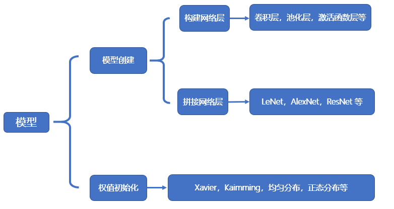
模型创建

创建模型有 2 个要素：构建子模块和拼接子模块。如 LeNet 里包含很多卷积层、池化层、全连接层，当我们构建好所有的子模块之后，按照一定的顺序拼接起来。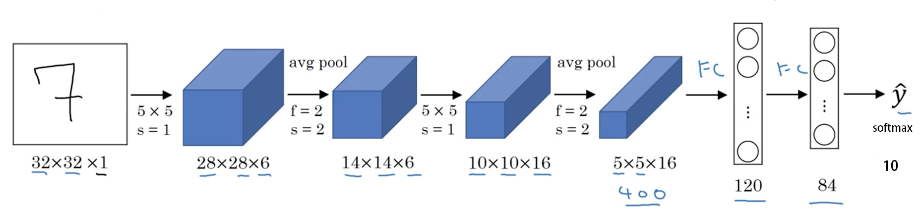

这里以上一篇文章中 lenet.py的 LeNet 为例，继承nn.Module，必须实现__init__() 方法和forward()方法。其中__init__() 方法里创建子模块，在forward()方法里拼接子模块。

class LeNet(nn.Module):
    # 子模块创建
    def __init__(self, classes):
        super(LeNet, self).__init__()
        self.conv1 = nn.Conv2d(3, 6, 5)
        self.conv2 = nn.Conv2d(6, 16, 5)
        self.fc1 = nn.Linear(16*5*5, 120)
        self.fc2 = nn.Linear(120, 84)
        self.fc3 = nn.Linear(84, classes)
    # 子模块拼接
    def forward(self, x):
        out = F.relu(self.conv1(x))
        out = F.max_pool2d(out, 2)
        out = F.relu(self.conv2(out))
        out = F.max_pool2d(out, 2)
        out = out.view(out.size(0), -1)
        out = F.relu(self.fc1(out))
        out = F.relu(self.fc2(out))
        out = self.fc3(out)
        return out

当我们调用net = LeNet(classes=2)创建模型时，会调用__init__()方法创建模型的子模块。

当我们在训练时调用outputs = net(inputs)时，会进入module.py的call()函数中：

def __call__(self, *input, **kwargs):
    for hook in self._forward_pre_hooks.values():
        result = hook(self, input)
        if result is not None:
            if not isinstance(result, tuple):
                result = (result,)
            input = result
    if torch._C._get_tracing_state():
        result = self._slow_forward(*input, **kwargs)
    else:
        result = self.forward(*input, **kwargs)
    ...
    ...
    ...

最终会调用result = self.forward(*input, **kwargs)函数，该函数会进入模型的forward()函数中，进行前向传播。

在 torch.nn中包含 4 个模块，如下图所示。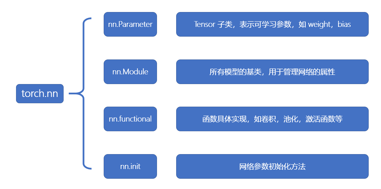

其中所有网络模型都是继承于nn.Module的，下面重点分析nn.Module模块。

nn.Module

nn.Module 有 8 个属性，都是OrderDict(有序字典)。在 LeNet 的__init__()方法中会调用父类nn.Module的__init__()方法，创建这 8 个属性。

def __init__(self):
    """
    Initializes internal Module state, shared by both nn.Module and ScriptModule.
    """
    torch._C._log_api_usage_once("python.nn_module")

    self.training = True
    self._parameters = OrderedDict()
    self._buffers = OrderedDict()
    self._backward_hooks = OrderedDict()
    self._forward_hooks = OrderedDict()
    self._forward_pre_hooks = OrderedDict()
    self._state_dict_hooks = OrderedDict()
    self._load_state_dict_pre_hooks = OrderedDict()
    self._modules = OrderedDict()

_parameters 属性：存储管理 nn.Parameter 类型的参数
_modules 属性：存储管理 nn.Module 类型的参数
_buffers 属性：存储管理缓冲属性，如 BN 层中的 running_mean
5 个 *_hooks 属性：存储管理钩子函数

其中比较重要的是parameters和modules属性。

在 LeNet 的__init__()中创建了 5 个子模块，nn.Conv2d()和nn.Linear()都是继承于nn.module，也就是说一个 module 都是包含多个子 module 的。

class LeNet(nn.Module):
    # 子模块创建
    def __init__(self, classes):
        super(LeNet, self).__init__()
        self.conv1 = nn.Conv2d(3, 6, 5)
        self.conv2 = nn.Conv2d(6, 16, 5)
        self.fc1 = nn.Linear(16*5*5, 120)
        self.fc2 = nn.Linear(120, 84)
        self.fc3 = nn.Linear(84, classes)
        ...
        ...
        ...

当调用net = LeNet(classes=2)创建模型后，net对象的 modules 属性就包含了这 5 个子网络模块。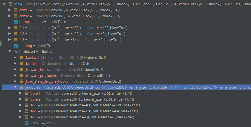

下面看下每个子模块是如何添加到 LeNet 的_modules 属性中的。以self.conv1 = nn.Conv2d(3, 6, 5)为例，当我们运行到这一行时，首先 Step Into 进入 Conv2d的构造，然后 Step Out。右键Evaluate Expression查看nn.Conv2d(3, 6, 5)的属性。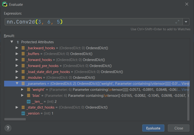

上面说了Conv2d也是一个 module，里面的_modules属性为空，_parameters属性里包含了该卷积层的可学习参数，这些参数的类型是 Parameter，继承自 Tensor。

此时只是完成了nn.Conv2d(3, 6, 5) module 的创建。还没有赋值给self.conv1。在nn.Module里有一个机制，会拦截所有的类属性赋值操作(self.conv1是类属性)，进入到__setattr__()函数中。我们再次 Step Into 就可以进入__setattr__()。

def __setattr__(self, name, value):
    def remove_from(*dicts):
        for d in dicts:
            if name in d:
                del d[name]

    params = self.__dict__.get('_parameters')
    if isinstance(value, Parameter):
        if params is None:
            raise AttributeError(
                "cannot assign parameters before Module.__init__() call")
        remove_from(self.__dict__, self._buffers, self._modules)
        self.register_parameter(name, value)
    elif params is not None and name in params:
        if value is not None:
            raise TypeError("cannot assign '{}' as parameter '{}' "
                            "(torch.nn.Parameter or None expected)"
                            .format(torch.typename(value), name))
        self.register_parameter(name, value)
    else:
        modules = self.__dict__.get('_modules')
        if isinstance(value, Module):
            if modules is None:
                raise AttributeError(
                    "cannot assign module before Module.__init__() call")
            remove_from(self.__dict__, self._parameters, self._buffers)
            modules[name] = value
        elif modules is not None and name in modules:
            if value is not None:
                raise TypeError("cannot assign '{}' as child module '{}' "
                                "(torch.nn.Module or None expected)"
                                .format(torch.typename(value), name))
            modules[name] = value
        ...
        ...
        ...

在这里判断 value 的类型是Parameter还是Module，存储到对应的有序字典中。

这里nn.Conv2d(3, 6, 5)的类型是Module，因此会执行modules[name] = value，key 是类属性的名字conv1，value 就是nn.Conv2d(3, 6, 5)。

总结

一个 module 里可包含多个子 module。比如 LeNet 是一个 Module，里面包括多个卷积层、池化层、全连接层等子 module
一个 module 相当于一个运算，必须实现 forward() 函数
每个 module 都有 8 个字典管理自己的属性
模型容器
除了上述的模块之外，还有一个重要的概念是模型容器 (Containers)，常用的容器有 3 个，这些容器都是继承自nn.Module。
nn.Sequetial：按照顺序包装多个网络层
nn.ModuleList：像 python 的 list 一样包装多个网络层，可以迭代
nn.ModuleDict：像 python 的 dict一样包装多个网络层，通过 (key, value) 的方式为每个网络层指定名称。
nn.Sequetial
在传统的机器学习中，有一个步骤是特征工程，我们需要从数据中人为地提取特征，然后把特征输入到分类器中预测。在深度学习的时代，特征工程的概念被弱化了，特征提取和分类器这两步被融合到了一个神经网络中。在卷积神经网络中，前面的卷积层以及池化层可以认为是特征提取部分，而后面的全连接层可以认为是分类器部分。比如 LeNet 就可以分为特征提取和分类器两部分，这 2 部分都可以分别使用 nn.Seuqtial 来包装。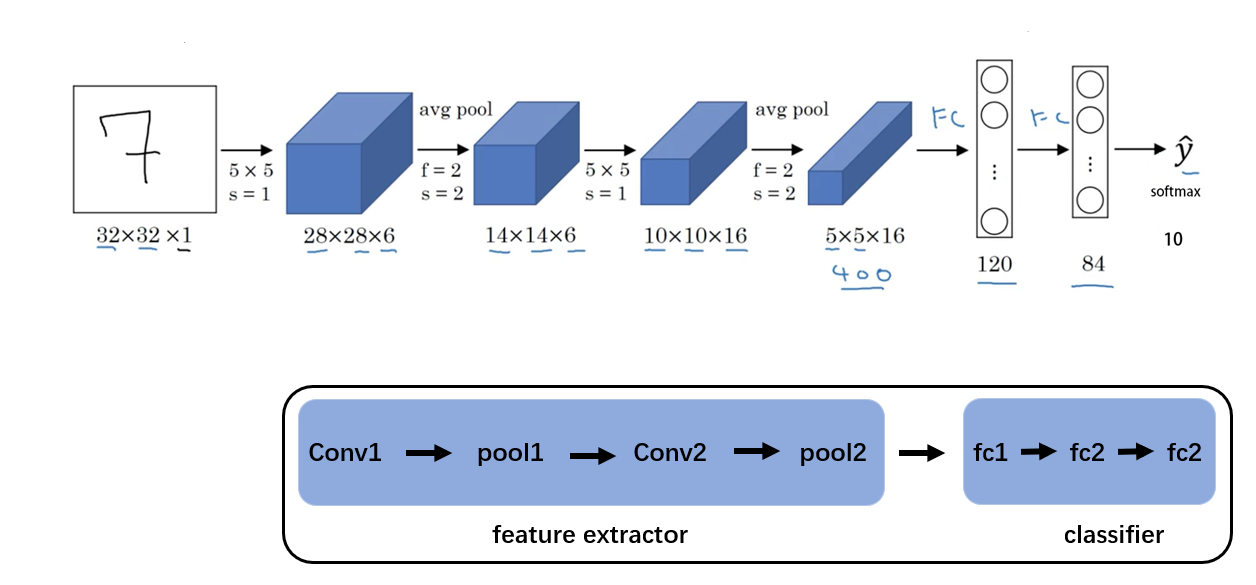

代码如下：

class LeNetSequetial(nn.Module):
    def __init__(self, classes):
        super(LeNet2, self).__init__()
        self.features = nn.Sequential(
            nn.Conv2d(3, 6, 5),
            nn.ReLU(),
            nn.AvgPool2d(2, 2),
            nn.Conv2d(6, 16, 5),
            nn.ReLU(),
            nn.AvgPool2d(2, 2)
        )
        self.classifier = nn.Sequential(
            nn.Linear(16*5*5, 120),
            nn.ReLU(),
            nn.Linear(120, 84),
            nn.ReLU(),
            nn.Linear(84, classes)
        )

    def forward(self, x):
        x = self.features(x)
        x = x.view(x.size()[0], -1)
        x = self.classifier(x)
        return x

在初始化时，nn.Sequetial会调用__init__()方法，将每一个子 module 添加到自身的_modules属性中。这里可以看到，我们传入的参数可以是一个 list，或者一个 OrderDict。如果是一个 OrderDict，那么则使用 OrderDict 里的 key，否则使用数字作为 key (OrderDict 的情况会在下面提及)。

def __init__(self, *args):
    super(Sequential, self).__init__()
    if len(args) == 1 and isinstance(args[0], OrderedDict):
        for key, module in args[0].items():
            self.add_module(key, module)
    else:
        for idx, module in enumerate(args):
            self.add_module(str(idx), module)

网络初始化完成后有两个子 module：features和classifier。

在进行前向传播时，会进入 LeNet 的forward()函数，首先调用第一个Sequetial容器：self.features，由于self.features也是一个 module，因此会调用__call__()函数，里面调用 result = self.forward(*input, **kwargs)，进入nn.Seuqetial的forward()函数，在这里依次调用所有的 module。

def forward(self, input):
    for module in self:
        input = module(input)
    return input

在nn.Sequetial中，里面的每个子网络层 module 是使用序号来索引的，即使用数字来作为 key。一旦网络层增多，难以查找特定的网络层，这种情况可以使用 OrderDict (有序字典)。代码中使用

class LeNetSequentialOrderDict(nn.Module):
    def __init__(self, classes):
        super(LeNetSequentialOrderDict, self).__init__()

        self.features = nn.Sequential(OrderedDict({
            'conv1': nn.Conv2d(3, 6, 5),
            'relu1': nn.ReLU(inplace=True),
            'pool1': nn.MaxPool2d(kernel_size=2, stride=2),

            'conv2': nn.Conv2d(6, 16, 5),
            'relu2': nn.ReLU(inplace=True),
            'pool2': nn.MaxPool2d(kernel_size=2, stride=2),
        }))

        self.classifier = nn.Sequential(OrderedDict({
            'fc1': nn.Linear(16*5*5, 120),
            'relu3': nn.ReLU(),

            'fc2': nn.Linear(120, 84),
            'relu4': nn.ReLU(inplace=True),

            'fc3': nn.Linear(84, classes),
        }))
        ...
        ...
        ...

总结
nn.Sequetial是nn.Module的容器，用于按顺序包装一组网络层，有以下两个特性。

顺序性：各网络层之间严格按照顺序构建，我们在构建网络时，一定要注意前后网络层之间输入和输出数据之间的形状是否匹配
自带forward()函数：在nn.Sequetial的forward()函数里通过 for 循环依次读取每个网络层，执行前向传播运算。这使得我们我们构建的模型更加简洁
nn.ModuleList
nn.ModuleList是nn.Module的容器，用于包装一组网络层，以迭代的方式调用网络层，主要有以下 3 个方法：
append()：在 ModuleList 后面添加网络层
extend()：拼接两个 ModuleList
insert()：在 ModuleList 的指定位置中插入网络层

下面的代码通过列表生成式来循环迭代创建 20 个全连接层，非常方便，只是在 forward()函数中需要手动调用每个网络层。

class ModuleList(nn.Module):
    def __init__(self):
        super(ModuleList, self).__init__()
        self.linears = nn.ModuleList([nn.Linear(10, 10) for i in range(20)])

    def forward(self, x):
        for i, linear in enumerate(self.linears):
            x = linear(x)
        return x


net = ModuleList()

print(net)

fake_data = torch.ones((10, 10))

output = net(fake_data)

print(output)

nn.ModuleDict

nn.ModuleDict是nn.Module的容器，用于包装一组网络层，以索引的方式调用网络层，主要有以下 5 个方法：

clear()：清空 ModuleDict
items()：返回可迭代的键值对 (key, value)
keys()：返回字典的所有 key
values()：返回字典的所有 value
pop()：返回一对键值，并从字典中删除

下面的模型创建了两个ModuleDict：self.choices和self.activations，在前向传播时通过传入对应的 key 来执行对应的网络层。

class ModuleDict(nn.Module):
    def __init__(self):
        super(ModuleDict, self).__init__()
        self.choices = nn.ModuleDict({
            'conv': nn.Conv2d(10, 10, 3),
            'pool': nn.MaxPool2d(3)
        })

        self.activations = nn.ModuleDict({
            'relu': nn.ReLU(),
            'prelu': nn.PReLU()
        })

    def forward(self, x, choice, act):
        x = self.choices[choice](x)
        x = self.activations[act](x)
        return x


net = ModuleDict()

fake_img = torch.randn((4, 10, 32, 32))

output = net(fake_img, 'conv', 'relu')
# output = net(fake_img, 'conv', 'prelu')
print(output)

容器总结

nn.Sequetial：顺序性，各网络层之间严格按照顺序执行，常用于 block 构建，在前向传播时的代码调用变得简洁
nn.ModuleList：迭代行，常用于大量重复网络构建，通过 for 循环实现重复构建
nn.ModuleDict：索引性，常用于可选择的网络层
卷积层
1D/2D/3D 卷积
卷积有一维卷积、二维卷积、三维卷积。一般情况下，卷积核在几个维度上滑动，就是几维卷积。比如在图片上的卷积就是二维卷积。
一维卷积
二维卷积
三维卷积
二维卷积：nn.Conv2d()
1
2
3
nn.Conv2d(self, in_channels, out_channels, kernel_size, stride=1, padding=0, dilation=1, groups=1, bias=True, padding_mode='zeros')
这个函数的功能是对多个二维信号进行二维卷积，主要参数如下：
in_channels：输入通道数
out_channels：输出通道数，等价于卷积核个数
kernel_size：卷积核尺寸
stride：步长
padding：填充宽度，主要是为了调整输出的特征图大小，一般把 padding 设置合适的值后，保持输入和输出的图像尺寸不变。
dilation：空洞卷积大小，默认为1，这时是标准卷积，常用于图像分割任务中，主要是为了提升感受野
groups：分组卷积设置，主要是为了模型的轻量化，如在 ShuffleNet、MobileNet、SqueezeNet中用到

bias：偏置

卷积尺寸计算

简化版卷积尺寸计算

这里不考虑空洞卷积，假设输入图片大小为 $I \times I$，卷积核大小为 $k \times k$，stride 为 $s$，padding 的像素数为 $p$，图片经过卷积之后的尺寸 $O$ 如下：
$O = \displaystyle\frac{I -k + 2 \times p}{s} +1$
下面例子的输入图片大小为 $5 \times 5$，卷积大小为 $3 \times 3$，stride 为 1，padding 为 0，所以输出图片大小为 $\displaystyle\frac{5 -3 + 2 \times 0}{1} +1 = 3$。

完整版卷积尺寸计算

完整版卷积尺寸计算考虑了空洞卷积，假设输入图片大小为 $I \times I$，卷积核大小为 $k \times k$，stride 为 $s$，padding 的像素数为 $p$，dilation 为 $d$，图片经过卷积之后的尺寸 $O$ 如下：。
$O = \displaystyle\frac{I - d \times (k-1) + 2 \times p -1}{s} +1$

卷积网络示例（非完整训练）

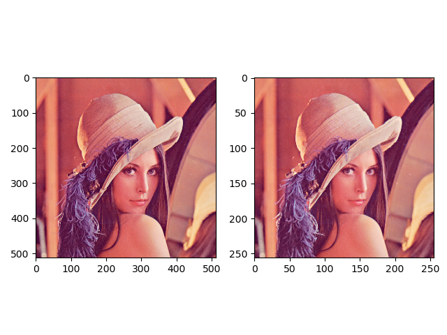
这里使用 inputchannel 为 3，output_channel 为 1 ，卷积核大小为 $3 \times 3$ 的卷积核nn.Conv2d(3, 1, 3)，使用nn.init.xavier_normal()方法初始化网络的权值。代码如下：

import os
import torch.nn as nn
from PIL import Image
from torchvision import transforms
from matplotlib import pyplot as plt
from common_tools import transform_invert, set_seed

set_seed(3)  # 设置随机种子

# ================================= load img ==================================
path_img = os.path.join(os.path.dirname(os.path.abspath(__file__)), "imgs", "lena.png")
print(path_img)
img = Image.open(path_img).convert('RGB')  # 0~255

# convert to tensor
img_transform = transforms.Compose([transforms.ToTensor()])
img_tensor = img_transform(img)
# 添加 batch 维度
img_tensor.unsqueeze_(dim=0)    # C*H*W to B*C*H*W

# ================================= create convolution layer ==================================

# ================ 2d
flag = 1
# flag = 0
if flag:
    conv_layer = nn.Conv2d(3, 1, 3)   # input:(i, o, size) weights:(o, i , h, w)
    # 初始化卷积层权值
    nn.init.xavier_normal_(conv_layer.weight.data)
    # nn.init.xavier_uniform_(conv_layer.weight.data)
    # calculation
    img_conv = conv_layer(img_tensor)

# ================ transposed
# flag = 1
flag = 0
if flag:
    conv_layer = nn.ConvTranspose2d(3, 1, 3, stride=2)   # input:(input_channel, output_channel, size)
    # 初始化网络层的权值
    nn.init.xavier_normal_(conv_layer.weight.data)

    # calculation
    img_conv = conv_layer(img_tensor)

# ================================= visualization ==================================
print("卷积前尺寸:{}\n卷积后尺寸:{}".format(img_tensor.shape, img_conv.shape))
img_conv = transform_invert(img_conv[0, 0:1, ...], img_transform)
img_raw = transform_invert(img_tensor.squeeze(), img_transform)
plt.subplot(122).imshow(img_conv, cmap='gray')
plt.subplot(121).imshow(img_raw)
plt.show()

卷积前后的图片如下 (左边是原图片，右边是卷积后的图片)：

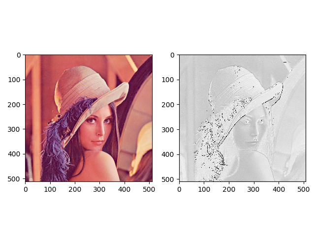
当改为使用nn.init.xavier_uniform_()方法初始化网络的权值时，卷积前后图片如下：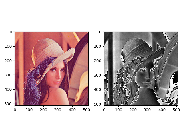

我们通过conv_layer.weight.shape查看卷积核的 shape 是(1, 3, 3, 3)，对应是(output_channel, input_channel, kernel_size, kernel_size)。所以第一个维度对应的是卷积核的个数，每个卷积核都是(3,3,3)。虽然每个卷积核都是 3 维的，执行的却是 2 维卷积。下面这个图展示了这个过程。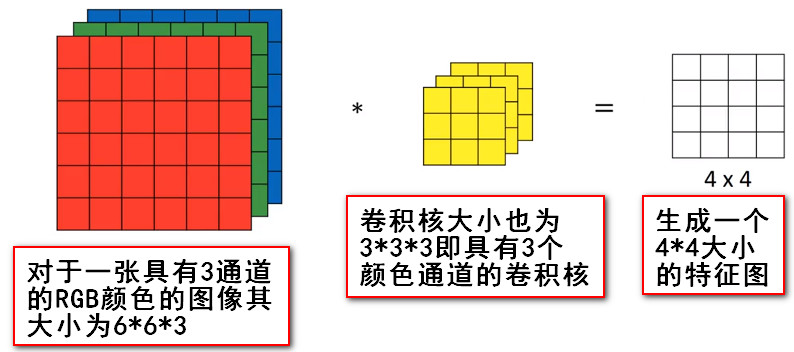

也就是每个卷积核在 input_channel 维度再划分，这里 input_channel 为 3，那么这时每个卷积核的 shape 是(3, 3)。3 个卷积核在输入图像的每个 channel 上卷积后得到 3 个数，把这 3 个数相加，再加上 bias，得到最后的一个输出。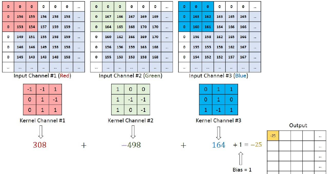

转置卷积：nn.ConvTranspose()

转置卷积又称为反卷积 (Deconvolution) 和部分跨越卷积 (Fractionally strided Convolution)，用于对图像进行上采样。
正常卷积如下：

原始的图片尺寸为 $4 \times 4$，卷积核大小为 $3 \times 3$，$padding =0$，$stride = 1$。由于卷积操作可以通过矩阵运算来解决，因此原始图片可以看作 $16 \times 1$ 的矩阵 $I{16 \times 1}$，卷积核可以看作 $4 \times 16$ 的矩阵$K{4 \times 16}$，那么输出是 $K{4 \times 16} \times I{16 \times 1} = O_{4 \times 1}$ 。
转置卷积如下：

原始的图片尺寸为 $2 \times 2$，卷积核大小为 $3 \times 3$，$padding =0$，$stride = 1$。由于卷积操作可以通过矩阵运算来解决，因此原始图片可以看作 $4 \times 1$ 的矩阵 $I{4 \times 1}$，卷积核可以看作 $4 \times 16$ 的矩阵$K{16 \times 4}$，那么输出是 $K{16 \times 4} \times I{4 \times 1} = O_{16 \times 1}$ 。
正常卷积核转置卷积矩阵的形状刚好是转置关系，因此称为转置卷积，但里面的权值不是一样的，卷积操作也是不可逆的。

PyTorch 中的转置卷积函数如下：

1
2
3

nn.ConvTranspose2d(self, in_channels, out_channels, kernel_size, stride=1,
                 padding=0, output_padding=0, groups=1, bias=True,
                 dilation=1, padding_mode='zeros')

和普通卷积的参数基本相同，不再赘述。

转置卷积尺寸计算

简化版转置卷积尺寸计算

这里不考虑空洞卷积，假设输入图片大小为 $ I \times I$，卷积核大小为 $k \times k$，stride 为 $s$，padding 的像素数为 $p$，图片经过卷积之后的尺寸 $ O $ 如下，刚好和普通卷积的计算是相反的：
$O = (I-1) \times s + k$

完整版简化版转置卷积尺寸计算

$O = (I-1) \times s - 2 \times p + d \times (k-1) + out_padding + 1$

转置卷积代码示例如下：

import os
import torch.nn as nn
from PIL import Image
from torchvision import transforms
from matplotlib import pyplot as plt
from common_tools import transform_invert, set_seed

set_seed(3)  # 设置随机种子

# ================================= load img ==================================
path_img = os.path.join(os.path.dirname(os.path.abspath(__file__)), "imgs", "lena.png")
print(path_img)
img = Image.open(path_img).convert('RGB')  # 0~255

# convert to tensor
img_transform = transforms.Compose([transforms.ToTensor()])
img_tensor = img_transform(img)
# 添加 batch 维度
img_tensor.unsqueeze_(dim=0)    # C*H*W to B*C*H*W

# ================================= create convolution layer ==================================

# ================ 2d
# flag = 1
flag = 0
if flag:
    conv_layer = nn.Conv2d(3, 1, 3)   # input:(i, o, size) weights:(o, i , h, w)
    # 初始化卷积层权值
    nn.init.xavier_normal_(conv_layer.weight.data)
    # nn.init.xavier_uniform_(conv_layer.weight.data)

    # calculation
    img_conv = conv_layer(img_tensor)

# ================ transposed
flag = 1
# flag = 0
if flag:
    conv_layer = nn.ConvTranspose2d(3, 1, 3, stride=2)   # input:(input_channel, output_channel, size)
    # 初始化网络层的权值
    nn.init.xavier_normal_(conv_layer.weight.data)

    # calculation
    img_conv = conv_layer(img_tensor)

# ================================= visualization ==================================
print("卷积前尺寸:{}\n卷积后尺寸:{}".format(img_tensor.shape, img_conv.shape))
img_conv = transform_invert(img_conv[0, 0:1, ...], img_transform)
img_raw = transform_invert(img_tensor.squeeze(), img_transform)
plt.subplot(122).imshow(img_conv, cmap='gray')
plt.subplot(121).imshow(img_raw)
plt.show()

转置卷积前后图片显示如下，左边原图片的尺寸是 (512, 512)，右边转置卷积后的图片尺寸是 (1025, 1025)。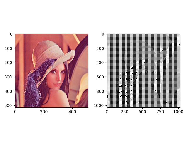

转置卷积后的图片一般都会有棋盘效应，像一格一格的棋盘，这是转置卷积的通病。

池化层、线性层和激活函数层

池化层

池化的作用则体现在降采样：保留显著特征、降低特征维度，增大kernel的感受野。另外一点值得注意：pooling也可以提供一些旋转不变性。池化层可对提取到的特征信息进行降维，一方面使特征图变小，简化网络计算复杂度并在一定程度上避免过拟合的出现；一方面进行特征压缩，提取主要特征。

有最大池化和平均池化两张方式。

最大池化：nn.MaxPool2d()

1	`nn.MaxPool2d(kernel_size, stride=None, padding=0, dilation=1, return_indices=False, ceil_mode=False)`

这个函数的功能是进行 2 维的最大池化，主要参数如下：

kernel_size：池化核尺寸
stride：步长，通常与 kernel_size 一致
padding：填充宽度，主要是为了调整输出的特征图大小，一般把 padding 设置合适的值后，保持输入和输出的图像尺寸不变。
dilation：池化间隔大小，默认为1。常用于图像分割任务中，主要是为了提升感受野
ceil_mode：默认为 False，尺寸向下取整。为 True 时，尺寸向上取整
return_indices：为 True 时，返回最大池化所使用的像素的索引，这些记录的索引通常在反最大池化时使用，把小的特征图反池化到大的特征图时，每一个像素放在哪个位置。

下图 (a) 表示反池化，(b) 表示上采样，(c) 表示反卷积。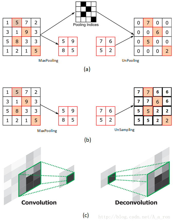

下面是最大池化的代码：

import os
import torch
import torch.nn as nn
from torchvision import transforms
from matplotlib import pyplot as plt
from PIL import Image
from common_tools import transform_invert, set_seed

set_seed(1)  # 设置随机种子

# ================================= load img ==================================
path_img = os.path.join(os.path.dirname(os.path.abspath(__file__)), "imgs/lena.png")
img = Image.open(path_img).convert('RGB')  # 0~255

# convert to tensor
img_transform = transforms.Compose([transforms.ToTensor()])
img_tensor = img_transform(img)
img_tensor.unsqueeze_(dim=0)    # C*H*W to B*C*H*W

# ================================= create convolution layer ==================================

# ================ maxpool
flag = 1
# flag = 0
if flag:
    maxpool_layer = nn.MaxPool2d((2, 2), stride=(2, 2))   # input:(i, o, size) weights:(o, i , h, w)
    img_pool = maxpool_layer(img_tensor)

print("池化前尺寸:{}\n池化后尺寸:{}".format(img_tensor.shape, img_pool.shape))
img_pool = transform_invert(img_pool[0, 0:3, ...], img_transform)
img_raw = transform_invert(img_tensor.squeeze(), img_transform)
plt.subplot(122).imshow(img_pool)
plt.subplot(121).imshow(img_raw)
plt.show()

结果如下：

1 2	`池化前尺寸:torch.Size([1, 3, 512, 512]) 池化后尺寸:torch.Size([1, 3, 256, 256])`

nn.AvgPool2d()

1	`torch.nn.AvgPool2d(kernel_size, stride=None, padding=0, ceil_mode=False, count_include_pad=True, divisor_override=None)`

这个函数的功能是进行 2 维的平均池化，主要参数如下：

kernel_size：池化核尺寸
stride：步长，通常与 kernel_size 一致
padding：填充宽度，主要是为了调整输出的特征图大小，一般把 padding 设置合适的值后，保持输入和输出的图像尺寸不变。
ilation：池化间隔大小，默认为1。常用于图像分割任务中，主要是为了提升感受野
ceil_mode：默认为 False，尺寸向下取整。为 True 时，尺寸向上取整
count_include_pad：在计算平均值时，是否把填充值考虑在内计算

divisor_override：除法因子。在计算平均值时，分子是像素值的总和，分母默认是像素值的个数。如果设置了 divisor_override，把分母改为 divisor_override。

img_tensor = torch.ones((1, 1, 4, 4))
avgpool_layer = nn.AvgPool2d((2, 2), stride=(2, 2))
img_pool = avgpool_layer(img_tensor)
print("raw_img:\n{}\npooling_img:\n{}".format(img_tensor, img_pool))

输出如下：

raw_img:
tensor([[[[1., 1., 1., 1.],
          [1., 1., 1., 1.],
          [1., 1., 1., 1.],
          [1., 1., 1., 1.]]]])
pooling_img:
tensor([[[[1., 1.],
          [1., 1.]]]])

加上divisor_override=3后，输出如下：

raw_img:
tensor([[[[1., 1., 1., 1.],
          [1., 1., 1., 1.],
          [1., 1., 1., 1.],
          [1., 1., 1., 1.]]]])
pooling_img:
tensor([[[[1.3333, 1.3333],
          [1.3333, 1.3333]]]])

nn.MaxUnpool2d()

1	`nn.MaxUnpool2d(kernel_size, stride=None, padding=0)`

功能是对二维信号（图像）进行最大值反池化，主要参数如下：

kernel_size：池化核尺寸
stride：步长，通常与 kernel_size 一致
padding：填充宽度

代码如下：

# pooling
img_tensor = torch.randint(high=5, size=(1, 1, 4, 4), dtype=torch.float)
maxpool_layer = nn.MaxPool2d((2, 2), stride=(2, 2), return_indices=True)
img_pool, indices = maxpool_layer(img_tensor)

# unpooling
img_reconstruct = torch.randn_like(img_pool, dtype=torch.float)
maxunpool_layer = nn.MaxUnpool2d((2, 2), stride=(2, 2))
img_unpool = maxunpool_layer(img_reconstruct, indices)

print("raw_img:\n{}\nimg_pool:\n{}".format(img_tensor, img_pool))
print("img_reconstruct:\n{}\nimg_unpool:\n{}".format(img_reconstruct, img_unpool))

输出如下：

# pooling
img_tensor = torch.randint(high=5, size=(1, 1, 4, 4), dtype=torch.float)
maxpool_layer = nn.MaxPool2d((2, 2), stride=(2, 2), return_indices=True)
img_pool, indices = maxpool_layer(img_tensor)

# unpooling
img_reconstruct = torch.randn_like(img_pool, dtype=torch.float)
maxunpool_layer = nn.MaxUnpool2d((2, 2), stride=(2, 2))
img_unpool = maxunpool_layer(img_reconstruct, indices)

print("raw_img:\n{}\nimg_pool:\n{}".format(img_tensor, img_pool))
print("img_reconstruct:\n{}\nimg_unpool:\n{}".format(img_reconstruct, img_unpool))

线性层

线性层又称为全连接层，其每个神经元与上一个层所有神经元相连，实现对前一层的线性组合或线性变换。
代码如下：

inputs = torch.tensor([[1., 2, 3]])
linear_layer = nn.Linear(3, 4)
linear_layer.weight.data = torch.tensor([[1., 1., 1.],
[2., 2., 2.],
[3., 3., 3.],
[4., 4., 4.]])

linear_layer.bias.data.fill_(0.5)
output = linear_layer(inputs)
print(inputs, inputs.shape)
print(linear_layer.weight.data, linear_layer.weight.data.shape)
print(output, output.shape)

输出为：

tensor([[1., 2., 3.]]) torch.Size([1, 3])
tensor([[1., 1., 1.],
        [2., 2., 2.],
        [3., 3., 3.],
        [4., 4., 4.]]) torch.Size([4, 3])
tensor([[ 6.5000, 12.5000, 18.5000, 24.5000]], grad_fn=<AddmmBackward>) torch.Size([1, 4])

激活函数层

假设第一个隐藏层为：$H{1}=X \times W{1}$，第二个隐藏层为：$H{2}=H{1} \times W_{2}$，输出层为：

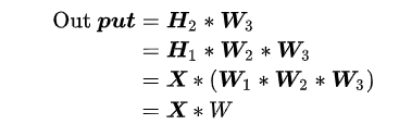
如果没有非线性变换，由于矩阵乘法的结合性，多个线性层的组合等价于一个线性层。

激活函数对特征进行非线性变换，赋予了多层神经网络具有深度的意义。下面介绍一些激活函数层。

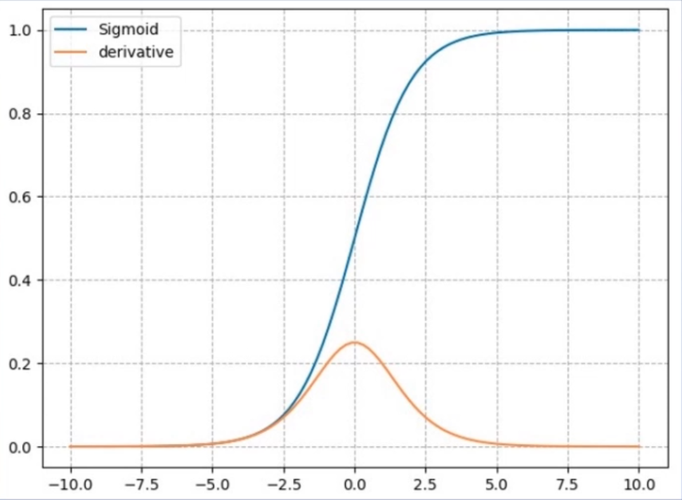
nn.Sigmoid

计算公式：$y=\frac{1}{1+e^{-x}}$
梯度公式：$y^{\prime}=y *(1-y)$
特性：
- 输出值在(0,1)，符合概率
- 导数范围是 [0, 0.25]，容易导致梯度消失
- 输出为非 0 均值，破坏数据分布
  nn.tanh
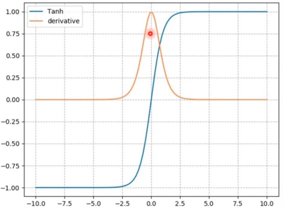
计算公式：$y=\frac{\sin x}{\cos x}=\frac{e^{x}-e^{-x}}{e^{-}+e^{-x}}=\frac{2}{1+e^{-2 x}}+1$
梯度公式：$y^{\prime}=1-y^{2}$
特性：
- 输出值在(-1, 1)，数据符合 0 均值
- 导数范围是 (0,1)，容易导致梯度消失
  nn.ReLU(修正线性单元)
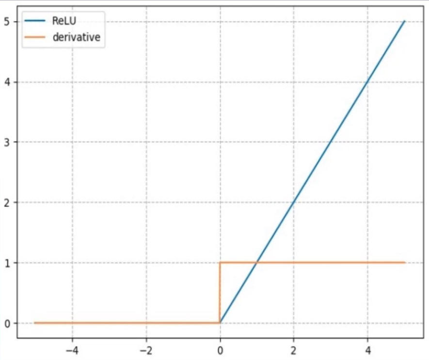
计算公式：$y=max(0, x)$
梯度公式：
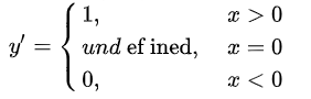
特性：
- 输出值均为正数，负半轴的导数为 0，容易导致死神经元
- 导数是 1，缓解梯度消失，但容易引发梯度爆炸
  
  针对 RuLU 会导致死神经元的缺点，出现了下面 3 种改进的激活函数。
  nn.LeakyReLU
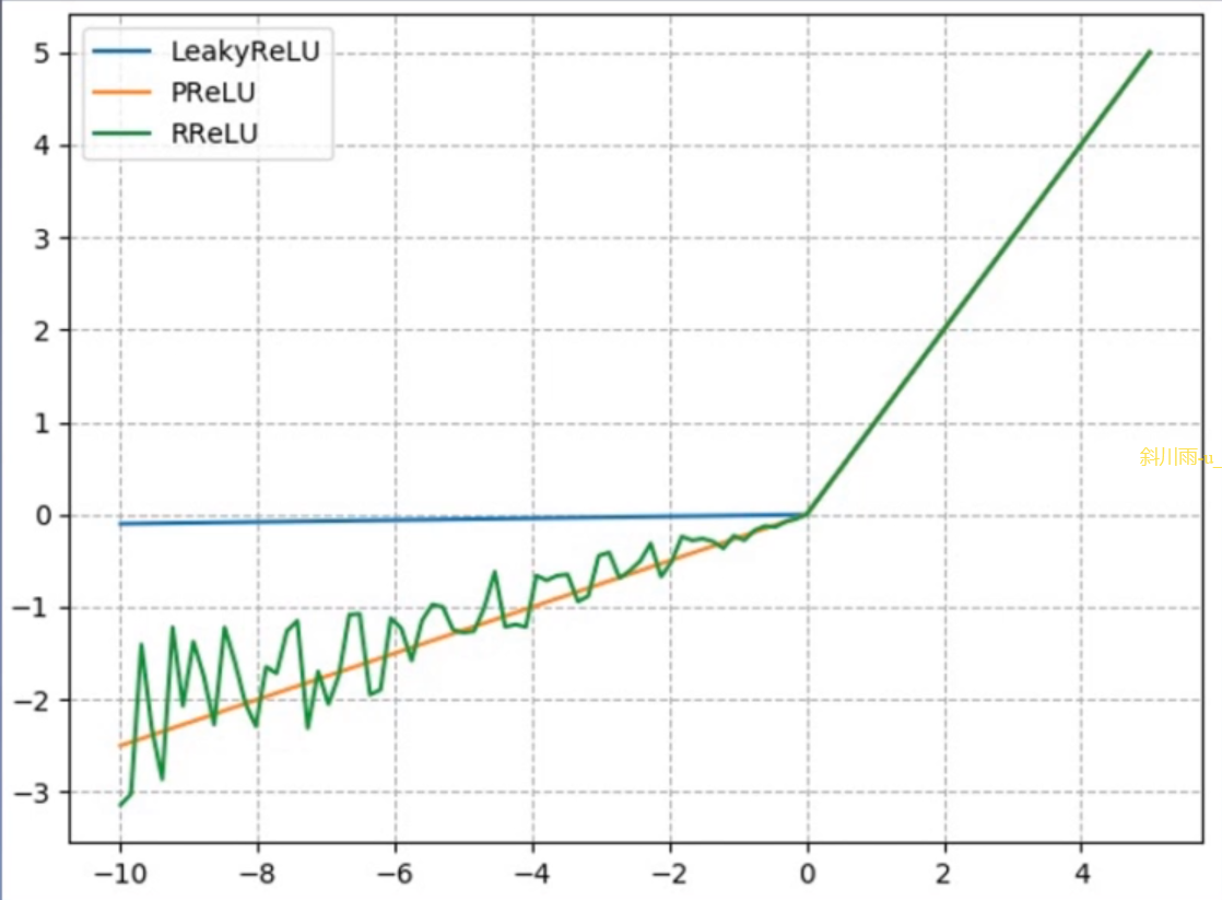
有一个参数negative_slope：设置负半轴斜率
nn.PReLU
有一个参数init：设置初始斜率，这个斜率是可学习的
nn.RReLU
R 是 random 的意思，负半轴每次斜率都是随机取 [lower, upper] 之间的一个数
lower：均匀分布下限
upper：均匀分布上限

深度学习

深度学习 pytorch

本博客所有文章除特别声明外，均采用 CC BY-NC-SA 4.0 协议，转载请注明出处！

深度学习-11-pytorch-4-损失函数与优化器上一篇

深度学习-9-pytorch-2-数据处理下一篇

模型创建

nn.Module

总结

模型容器

nn.Sequetial

nn.ModuleList

nn.ModuleDict

容器总结

卷积层

1D/2D/3D 卷积

一维卷积

二维卷积

三维卷积

二维卷积：nn.Conv2d()