本文最后更新于:2021年8月15日 下午
创作声明:主要内容参考于张贤同学https://zhuanlan.zhihu.com/p/265394674
Regularization Regularization 中文是正则化,可以理解为一种减少方差的策略。
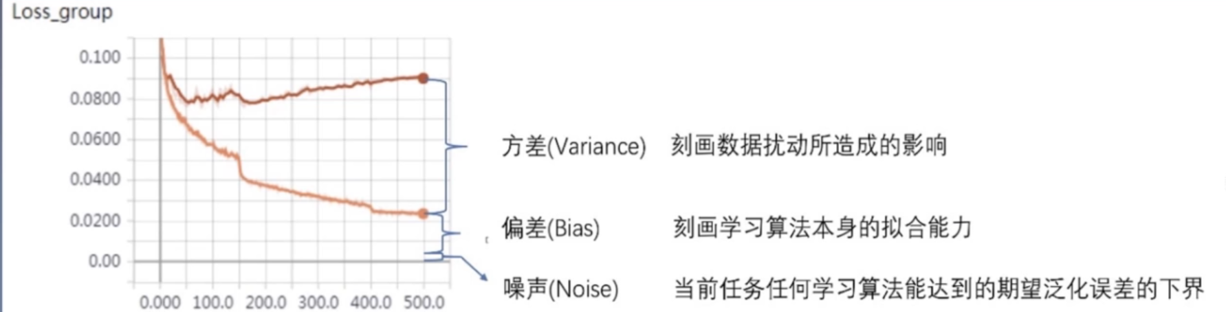
在机器学习中,误差可以分解为:偏差,方差与噪声之和。即误差=偏差+方差+噪声
偏差度量了学习算法的期望预测与真实结果的偏离程度,即刻画了学习算法本身的拟合能力。
方差度量了同样大小的训练集的变动所导致的学习性能的变化,即刻画了数据扰动所造成的影响。
噪声则表达了在当前任务上学习任何算法所能达到的期望泛化误差的下界。
当没有正则项时:$\boldsymbol{O} \boldsymbol{b} \boldsymbol{j}=\boldsymbol{L} \boldsymbol{o} \boldsymbol{s} \boldsymbol{s}$,$w_{i+1}=w_{i}-\frac{\partial o b j}{\partial w_{i}}=w_{i}-\frac{\partial L o s s}{\partial w_{i}}$。
当使用 L2 正则项时,$\boldsymbol{O} \boldsymbol{b} \boldsymbol{j}=\boldsymbol{L} \boldsymbol{o} \boldsymbol{s} \boldsymbol{s}+\frac{\lambda}{2} \sum{i}^{N} \boldsymbol{w}{i}^{2}$,$\begin{aligned} w{i+1}=w{i}-\frac{\partial o b j}{\partial w{i}} &=w{i}-\left(\frac{\partial L o s s}{\partial w_{i}}+\lambda w{i}\right) =w{i}(1-\lambda)-\frac{\partial L o s s}{\partial w_{i}} \end{aligned}$,其中$0 < \lambda < 1$,所以具有权值衰减的作用。
weight decay 在 PyTorch 中,L2 正则项是在优化器中实现的,在构造优化器时可以传入 weight decay 参数,对应的是公式中的$\lambda $。
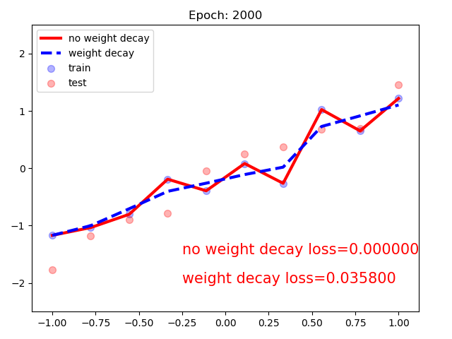
下面代码对比了没有 weight decay 的优化器和 weight decay 为 0.01 的优化器的训练情况,在线性回归的数据集上进行实验,模型使用 3 层的全连接网络,并使用 TensorBoard 可视化每层权值的变化情况。代码如下:
1
2
3
4
5
6
7
8
9
10
11
12
13
14
15
16
17
18
19
20
21
22
23
24
25
26
27
28
29
30
31
32
33
34
35
36
37
38
39
40
41
42
43
44
45
46
47
48
49
50
51
52
53
54
55
56
57
58
59
60
61
62
63
64
65
66
67
68
69
70
71
72
73
74
75
76
77
78
79
80
81
82
83
84
85
86
87
88
89
90
91
92
93
94
95
96
97
98
99
100
import torchfrom common_tools import set_seedfrom tensorboardX import SummaryWriternum_data =10, x_range=(-1, 1)):size =train_x.size())size =test_x.size())inplace =True ),inplace =True ),inplace =True ),neural_num =n_hidden)neural_num =n_hidden)lr =lr_init, momentum =0.9)lr =lr_init, momentum =0.9, weight_decay =1e-2)comment ='_test_tensorboard' , filename_suffix ="12345678" )for epoch in range(max_iter):step ()step ()if (epoch+1) % disp_interval == 0:for name, layer in net_normal.named_parameters():'_grad_normal' , layer.grad, epoch)'_data_normal' , layer, epoch)for name, layer in net_weight_decay.named_parameters():'_grad_weight_decay' , layer.grad, epoch)'_data_weight_decay' , layer, epoch)c ='blue' , s =50, alpha =0.3, label ='train' )c ='red' , s =50, alpha =0.3, label ='test' )'r-' , lw =3, label ='no weight decay' )'b--' , lw =3, label ='weight decay' )'no weight decay loss={:.6f}' .format(loss_normal.item()), fontdict={'size' : 15, 'color' : 'red' })'weight decay loss={:.6f}' .format(loss_wdecay.item()), fontdict={'size' : 15, 'color' : 'red' })loc ='upper left' )"Epoch: {}" .format(epoch+1))
训练 2000 个 epoch 后,模型如下:
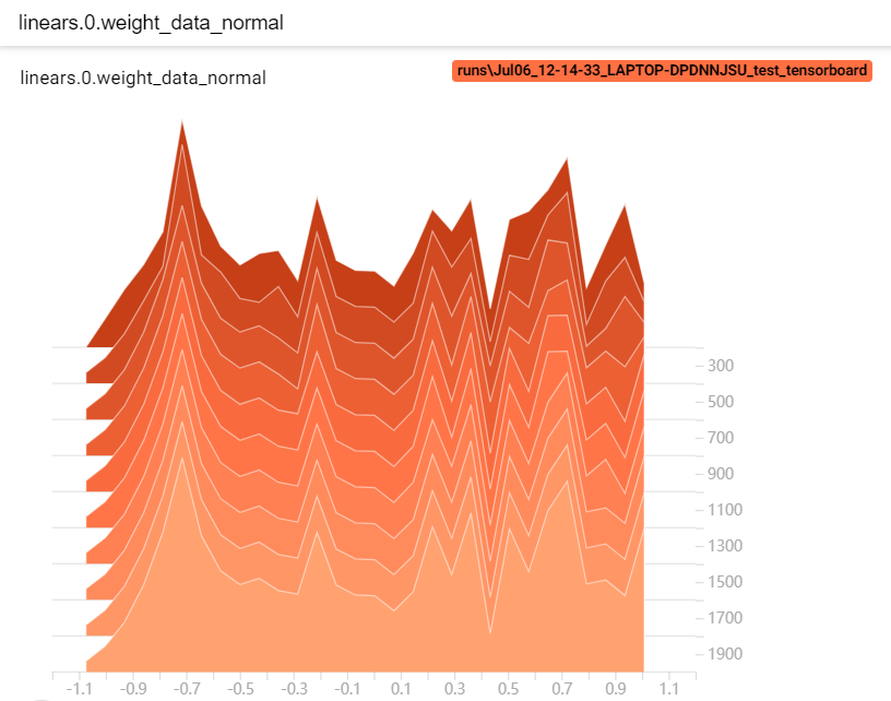
下面是使用 Tensorboard 可视化的分析。首先查看不带 weight decay 的权值变化过程,第一层权值变化如下:
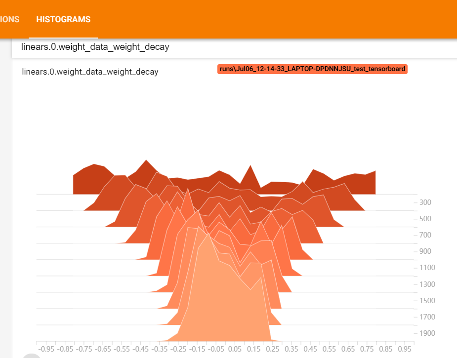
然后查看带 weight decay 的权值变化过程,第一层权值变化如下:
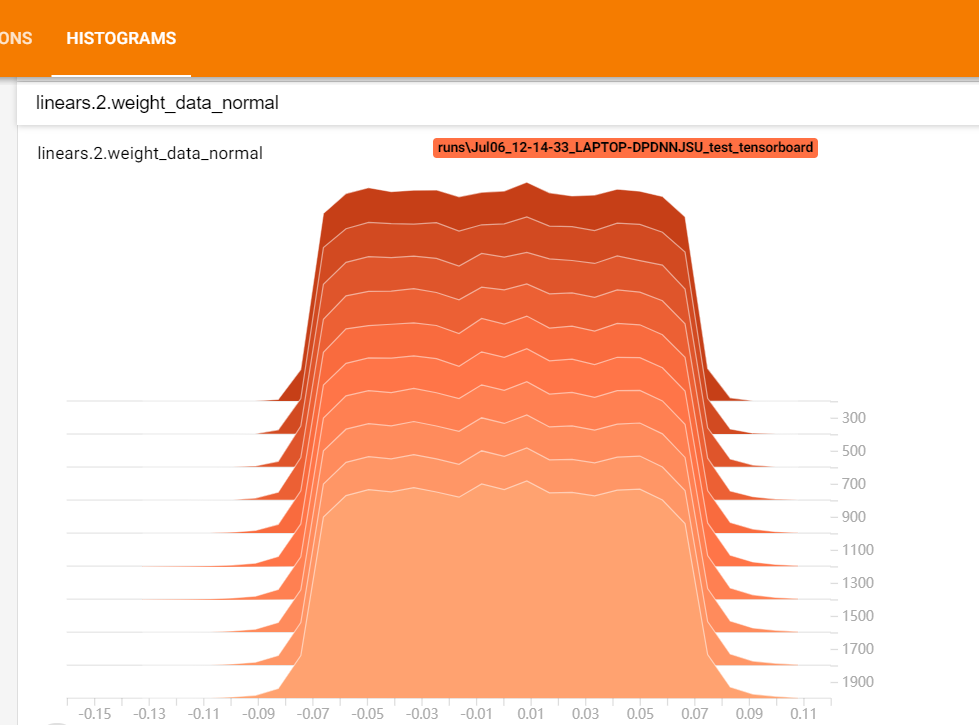
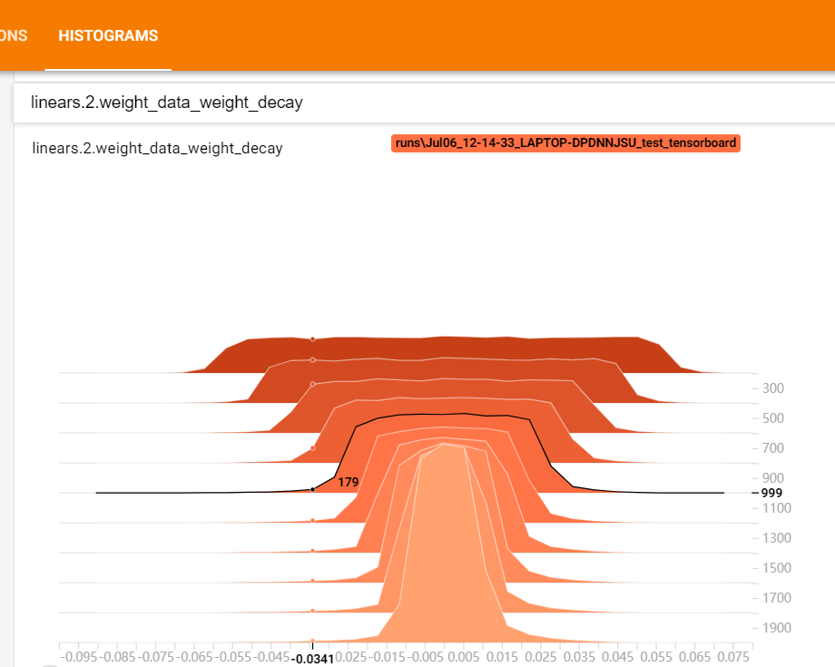
第二层不带 weight decay 的权值变化如下:
由于 weight decay 是在优化器的一个参数,因此在执行optim_wdecay.step()时,会计算 weight decay 后的梯度,具体代码如下:
1
2
3
4
5
6
7
8
9
10
11
12
13
14
15
16
17
18
19
20
21
22
23
24
25
26
27
def step (self, closure=None ):"""Performs a single optimization step. Arguments: closure (callable, optional): A closure that reevaluates the model and returns the loss. """ None if closure is not None :for group in self.param_groups:'weight_decay' ]'momentum' ]'dampening' ]'nesterov' ]for p in group['params' ]:if p.grad is None :continue if weight_decay != 0 :'lr' ], d_p)
可以看到:d_p 是计算得到的梯度,如果 weight decay 不为 0,那么更新 $d_p=dp+weight_decay \times p.data$,对应公式:$\left(\frac{\partial L o s s}{\partial w_{i}}+\lambda * w_{i}\right)$。最后一行是根据梯度更新权值。
Dropout Dropout 是另一种抑制过拟合的方法。在使用 dropout 时,数据尺度会发生变化,如果设置 dropout_prob =0.3,那么在训练时,数据尺度会变为原来的 70%;而在测试时,执行了 model.eval() 后,dropout 是关闭的,因此所有权重需要乘以 (1-dropout_prob),把数据尺度也缩放到 70%。
PyTorch 中 Dropout 层如下,通常放在每个网路层的最前面:
1 torch.nn.Dropout(p =0.5, inplace =False )
参数:
p:主力需要注意的是,p 是被舍弃的概率,也叫失活概率
下面实验使用的依然是线性回归的例子,两个网络均是 3 层的全连接层,每层前面都设置 dropout,一个网络的 dropout 设置为 0,另一个网络的 dropout 设置为 0.5,并使用 TensorBoard 可视化每层权值的变化情况。代码如下:
1
2
3
4
5
6
7
8
9
10
11
12
13
14
15
16
17
18
19
20
21
22
23
24
25
26
27
28
29
30
31
32
33
34
35
36
37
38
39
40
41
42
43
44
45
46
47
48
49
50
51
52
53
54
55
56
57
58
59
60
61
62
63
64
65
66
67
68
69
70
71
72
73
74
75
76
77
78
79
80
81
82
83
84
85
86
87
88
89
90
91
92
93
94
95
96
97
98
99
100
101
102
103
104
105
106
107
108
109
110
111
112
import torchfrom common_tools import set_seedfrom tensorboardX import SummaryWriternum_data =10, x_range=(-1, 1)):size =train_x.size())size =test_x.size())d_prob =0.5):inplace =True ),inplace =True ),inplace =True ),neural_num =n_hidden, d_prob =0.)neural_num =n_hidden, d_prob =0.5)lr =lr_init, momentum =0.9)lr =lr_init, momentum =0.9)comment ='_test_tensorboard' , filename_suffix ="12345678" )for epoch in range(max_iter):step ()step ()if (epoch+1) % disp_interval == 0:for name, layer in net_prob_0.named_parameters():'_grad_normal' , layer.grad, epoch)'_data_normal' , layer, epoch)for name, layer in net_prob_05.named_parameters():'_grad_regularization' , layer.grad, epoch)'_data_regularization' , layer, epoch)c ='blue' , s =50, alpha =0.3, label ='train' )c ='red' , s =50, alpha =0.3, label ='test' )'r-' , lw =3, label ='d_prob_0' )'b--' , lw =3, label ='d_prob_05' )'d_prob_0 loss={:.8f}' .format(loss_normal.item()), fontdict={'size' : 15, 'color' : 'red' })'d_prob_05 loss={:.6f}' .format(loss_wdecay.item()), fontdict={'size' : 15, 'color' : 'red' })loc ='upper left' )"Epoch: {}" .format(epoch+1))
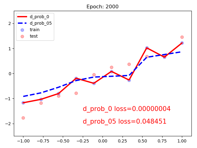
训练 2000 次后,模型的曲线如下:
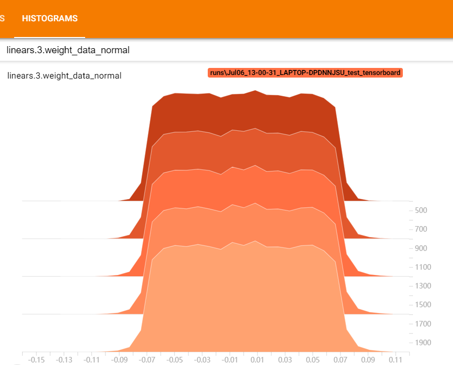
dropout =0 的权值变化如下:
model.eval() 和 model.trian() 有些网络层在训练状态和测试状态是不一样的,如 dropout 层,在训练时 dropout 层是有效的,但是数据尺度会缩放,为了保持数据尺度不变,所有的权重需要除以 1-p。而在测试时 dropout 层是关闭的。因此在测试时需要先调用model.eval()设置各个网络层的的training属性为 False,在训练时需要先调用model.train()设置各个网络层的的training属性为 True。
下面是对比 dropout 层的在 eval 和 train 模式下的输出值。
首先构造一层全连接网络,输入是 10000 个神经元,输出是 1 个神经元,权值全设为 1,dropout 设置为 0.5。输入是全为 1 的向量。分别测试网络在 train 模式和 eval 模式下的输出,代码如下:
1
2
3
4
5
6
7
8
9
10
11
12
13
14
15
16
17
18
19
20
21
22
23
24
25
26
27
28
29
30
import torch.nn as nn.Module ):__init__ (self, neural_num, d_prob=0.5 ):super (Net, self).__init__ ()Sequential (Dropout (d_prob),Linear (neural_num, 1 , bias=False),ReLU (inplace=True)forward (self, x):linears (x)10000 ones ((input_num, ), dtype=torch.float32)Net (input_num, d_prob=0.5 )1 ].weight.detach ().fill_ (1 .)train ()net (x)print ("output in training mode" , y)eval ()net (x)print ("output in eval mode" , y)
输出如下:
1
2
output in training mode tensor([9868 .], grad_fn=<ReluBackward1> )eval mode tensor([10000 .], grad_fn=<ReluBackward1> )
在训练时,由于 dropout 为 0.5,因此理论上输出值是 5000,而由于在训练时,dropout 层会把权值除以 1-p=0.5,也就是乘以 2,因此在 train 模式的输出是10000 附近的数(上下随机浮动是由于概率的不确定性引起的) 。而在 eval 模式下,关闭了 dropout,因此输出值是 10000。这种方式在训练时对权值进行缩放,在测试时就不用对权值进行缩放,加快了测试的速度。
Batch Normalization 称为批标准化。批是指一批数据,通常为 mini-batch;标准化是处理后的数据服从$N(0,1)$的正态分布。
批标准化的优点有如下:
可以使用更大的学习率,加速模型收敛
可以不用精心设计权值初始化
可以不用 dropout 或者较小的 dropout
可以不用 L2 或者较小的 weight decay
可以不用 LRN (local response normalization)
假设输入的 mini-batch 数据是
求 mini-batch 的均值:$\mu_{\mathcal{B}} \leftarrow \frac{1}{m} \sum_{i=1}^{m} x_{i}$
求 mini-batch 的方差:$\sigma_{\mathcal{B}}^{2} \leftarrow \frac{1}{m} \sum_{i=1}\left(x_{i}-\mu_{\mathcal{B}}\right)^{2}$
标准化:$\widehat{x}{i} \leftarrow \frac{x{i}-\mu{\mathcal{B}}}{\sqrt{\sigma{B}^{2}+\epsilon}}$,其中$\epsilon$ 是放置分母为 0 的一个数
affine transform(缩放和平移):$y{i} \leftarrow \gamma \widehat{x}{i}+\beta \equiv \mathrm{B} \mathrm{N}{\gamma, \beta}\left(x{i}\right)$,这个操作可以增强模型的 capacity,也就是让模型自己判断是否要对数据进行标准化,进行多大程度的标准化。如果$\gamma= \sqrt{\sigma_{B}^{2}}$,$\beta=\mu_{\mathcal{B}}$,那么就实现了恒等映射。
Batch Normalization 的提出主要是为了解决 Internal Covariate Shift (ICS)。在训练过程中,数据需要经过多层的网络,如果数据在前向传播的过程中,尺度发生了变化,可能会导致梯度爆炸或者梯度消失,从而导致模型难以收敛。
Batch Normalization 层一般在激活函数前一层。
下面的代码打印一个网络的每个网络层的输出,在没有进行初始化时,数据尺度越来越小。
1
2
3
4
5
6
7
8
9
10
11
12
13
14
15
16
17
18
19
20
21
22
23
24
25
26
27
28
29
30
31
32
33
34
35
36
37
38
39
40
41
42
43
44
45
46
47
48
49
50
51
52
import torchimport numpy as npimport torch.nn as nnfrom common_tools import set_seed1 ) class MLP (nn.Module ):def __init__ (self, neural_num, layers=100 ):super (MLP, self).__init__()False ) for i in range (layers)])for i in range (layers)])def forward (self, x ):for (i, linear), bn in zip (enumerate (self.linears), self.bns):if torch.isnan(x.std()):print ("output is nan in {} layers" .format (i))break print ("layers:{}, std:{}" .format (i, x.std().item()))return xdef initialize (self ):for m in self.modules():if isinstance (m, nn.Linear):256 100 16 print (output)
当使用nn.init.kaiming_normal_()初始化后,数据的标准差尺度稳定在 [0.6, 0.9]。
当我们不对网络层进行权值初始化,而是在每个激活函数层之前使用 bn 层,查看数据的标准差尺度稳定在 [0.58, 0.59]。因此 Batch Normalization 可以不用精心设计权值初始化。
下面以人民币二分类实验中的 LeNet 为例,添加 bn 层,对比不带 bn 层的网络和带 bn 层的网络的训练过程。
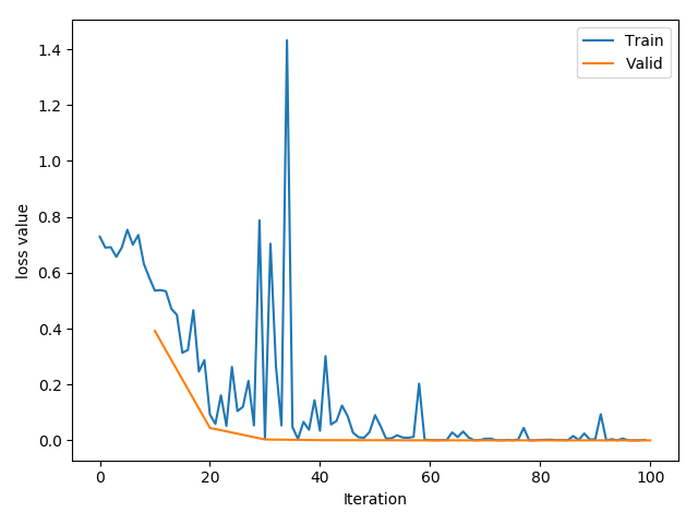
不带 bn 层的网络,并且使用 kaiming 初始化权值,训练过程如下:
带有 bn 层的 LeNet 定义如下:
1
2
3
4
5
6
7
8
9
10
11
12
13
14
15
16
17
18
19
20
21
22
23
24
25
26
27
28
29
30
31
32
33
34
35
36
37
class LeNet_bn (nn .Module ):def __init__ self , classes):super (LeNet_bn, self ).__init__()self .conv1 = nn.Conv2d(3 , 6 , 5 )self .bn1 = nn.BatchNorm2d(num_features=6 )self .conv2 = nn.Conv2d(6 , 16 , 5 )self .bn2 = nn.BatchNorm2d(num_features=16 )self .fc1 = nn.Linear(16 * 5 * 5 , 120 )self .bn3 = nn.BatchNorm1d(num_features=120 )self .fc2 = nn.Linear(120 , 84 )self .fc3 = nn.Linear(84 , classes)def forward self , x):out = self .conv1(x)out = self .bn1(out )out = F.relu(out )out = F.max_pool2d(out , 2 )out = self .conv2(out )out = self .bn2(out )out = F.relu(out )out = F.max_pool2d(out , 2 )out = out .view(out .size(0 ), -1 )out = self .fc1(out )out = self .bn3(out )out = F.relu(out )out = F.relu(self .fc2(out ))out = self .fc3(out )return out
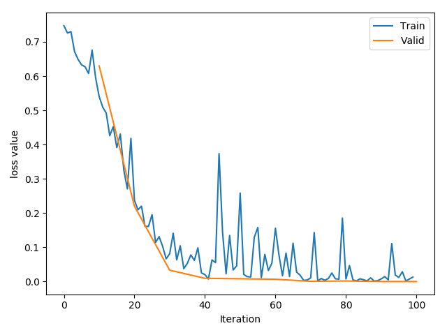
带 bn 层的网络,并且不使用 kaiming 初始化权值,训练过程如下:
Batch Normalization in PyTorch 在 PyTorch 中,有 3 个 Batch Normalization 类
nn.BatchNorm1d(),输入数据的形状是 $B \times C \times 1D_feature$
nn.BatchNorm2d(),输入数据的形状是 $B \times C \times 2D_feature$
nn.BatchNorm3d(),输入数据的形状是 $B \times C \times 3D_feature$
以nn.BatchNorm1d()为例,如下:
1 torch.nn.BatchNorm1d(num_features, eps =1e-05, momentum =0.1, affine =True , track_running_stats =True )
参数:
num_features:一个样本的特征数量,这个参数最重要
eps:在进行标准化操作时的分布修正项
momentum:指数加权平均估计当前的均值和方差
affine:是否需要 affine transform,默认为 True
track_running_stats:True 为训练状态,此时均值和方差会根据每个 mini-batch 改变。False 为测试状态,此时均值和方差会固定
主要属性:
runninng_mean:均值
running_var:方差
weight:affine transform 中的 $\gamma$
bias:affine transform 中的 $\beta$
在训练时,均值和方差采用指数加权平均计算,也就是不仅考虑当前 mini-batch 的值均值和方差还考虑前面的 mini-batch 的均值和方差。
在训练时,均值方差固定为当前统计值。
所有的 bn 层都是根据特征维度 计算上面 4 个属性,详情看下面例子。
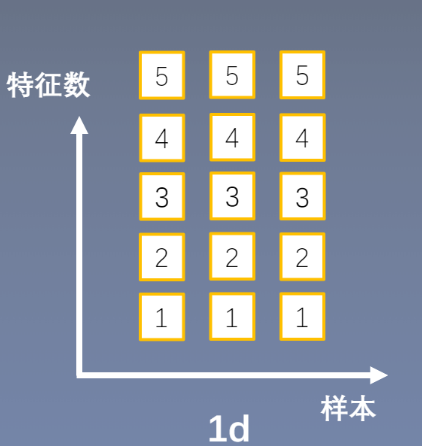
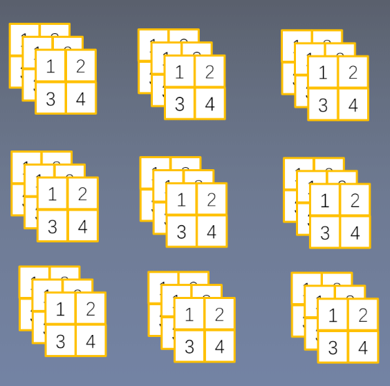
nn.BatchNorm1d() 输入数据的形状是 $B \times C \times 1D_feature$。在下面的例子中,数据的维度是:(3, 5, 1),表示一个 mini-batch 有 3 个样本,每个样本有 5 个特征,每个特征的维度是 1。那么就会计算 5 个均值和方差,分别对应每个特征维度。momentum 设置为 0.3,第一次的均值和方差默认为 0 和 1。输入两次 mini-batch 的数据。
数据如下图:
1
2
3
4
5
6
7
8
9
10
11
12
13
14
15
16
17
18
19
20
21
22
23
24
25
26
27
28
batch_size = 3 num_features = 5 momentum = 0.3 features_shape = (1 )feature_map = torch.ones(features_shape) feature_maps = torch.stack([feature_map*(i+1 ) for i in range(num_features)], dim=0) feature_maps_bs = torch.stack([feature_maps for i in range(batch_size)], dim=0) "input data:\n{} shape is {}" .format(feature_maps_bs, feature_maps_bs.shape))bn = nn.BatchNorm1d(num_features=num_features, momentum=momentum) running_var = 0 , 1 var_t = 2 , 0 in range(2 ):outputs = bn(feature_maps_bs)"\niteration:{}, running mean: {} " .format(i, bn.running_mean))"iteration:{}, running var:{} " .format(i, bn.running_var))running_mean = (1 - momentum) * running_mean + momentum * mean_trunning_var = (1 - momentum) * running_var + momentum * var_t"iteration:{}, 第二个特征的running mean: {} " .format(i, running_mean))"iteration:{}, 第二个特征的running var:{}" .format(i, running_var))
输出为:
1
2
3
4
5
6
7
8
9
10
11
12
13
14
15
16
17
18
19
20
21
22
23
24
input data:[[[1.] ,[2.] ,[3.] ,[4.] ,[5.] ],[[1.] ,[2.] ,[3.] ,[4.] ,[5.] ],[[1.] ,[2.] ,[3.] ,[4.] ,[5.] ]]) shape is torch.Size ([3, 5, 1] )0 , running mean: tensor([0.3000, 0.6000, 0.9000, 1.2000, 1.5000] ) 0 , running var :tensor([0.7000, 0.7000, 0.7000, 0.7000, 0.7000] ) 0 , 第二个特征的running mean: 0.6 0 , 第二个特征的running var :0.7 1 , running mean: tensor([0.5100, 1.0200, 1.5300, 2.0400, 2.5500] ) 1 , running var :tensor([0.4900, 0.4900, 0.4900, 0.4900, 0.4900] ) 1 , 第二个特征的running mean: 1.02 1 , 第二个特征的running var :0.48999999999999994
虽然两个 mini-batch 的数据是一样的,但是 bn 层的均值和方差却不一样。以第二个特征的均值计算为例,值都是 2。
第一次 bn 层的均值计算:$running_mean=(1-momentum) \times pre_running_mean + momentum \times mean_t =(1-0.3) \times 0 + 0.3 \times 2 =0.6$
第二次 bn 层的均值计算:$running_mean=(1-momentum) \times pre_running_mean + momentum \times mean_t =(1-0.3) \times 0.6 + 0.3 \times 2 =1.02$
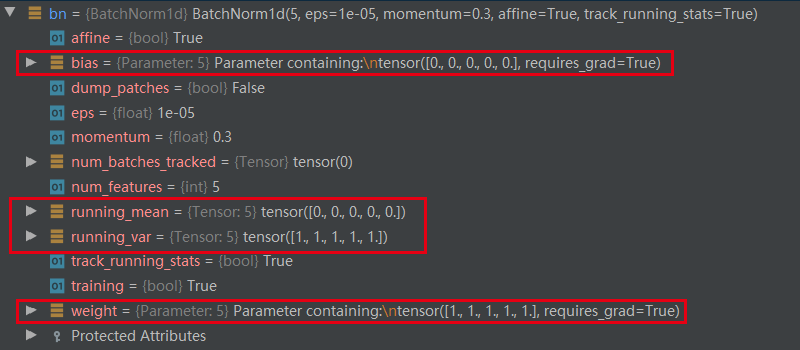
网络还没进行前向传播之前,断点查看 bn 层的属性如下:
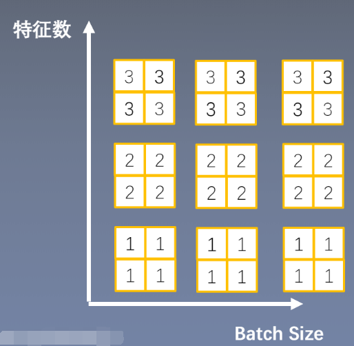
nn.BatchNorm2d() 输入数据的形状是 $B \times C \times 2D_feature$。在下面的例子中,数据的维度是:(3, 3, 2, 2),表示一个 mini-batch 有 3 个样本,每个样本有 3 个特征,每个特征的维度是 $1 \times 2$。那么就会计算 3 个均值和方差,分别对应每个特征维度。momentum 设置为 0.3,第一次的均值和方差默认为 0 和 1。输入两次 mini-batch 的数据。
数据如下图:
1
2
3
4
5
6
7
8
9
10
11
12
13
14
15
16
17
18
19
20
21
22
23
24
batch_size = 3 num_features = 3 momentum = 0.3 features_shape = (2 , 2 )feature_map = torch.ones(features_shape) feature_maps = torch.stack([feature_map*(i+1 ) for i in range(num_features)], dim=0) feature_maps_bs = torch.stack([feature_maps for i in range(batch_size)], dim=0) bn = nn.BatchNorm2d(num_features=num_features, momentum=momentum) running_var = 0 , 1 in range(2 ):outputs = bn(feature_maps_bs)"\niter:{}, running_mean: {}" .format(i, bn.running_mean))"iter:{}, running_var: {}" .format(i, bn.running_var))"iter:{}, weight: {}" .format(i, bn.weight.data.numpy()))"iter:{}, bias: {}" .format(i, bn.bias.data.numpy()))
输出如下:
1
2
3
4
5
6
7
8
iter :0 , running_mean: tensor([0 .3000 , 0 .6000 , 0 .9000 ])iter :0 , running_var: tensor([0 .7000 , 0 .7000 , 0 .7000 ])iter :0 , weight: [1. 1. 1.] iter :0 , bias: [0. 0. 0.] iter :1 , running_mean: tensor([0 .5100 , 1 .0200 , 1 .5300 ])iter :1 , running_var: tensor([0 .4900 , 0 .4900 , 0 .4900 ])iter :1 , weight: [1. 1. 1.] iter :1 , bias: [0. 0. 0.]
nn.BatchNorm3d() 输入数据的形状是 $B \times C \times 3D_feature$。在下面的例子中,数据的维度是:(3, 2, 2, 2, 3),表示一个 mini-batch 有 3 个样本,每个样本有 2 个特征,每个特征的维度是 $2 \times 2 \times 3$。那么就会计算 2 个均值和方差,分别对应每个特征维度。momentum 设置为 0.3,第一次的均值和方差默认为 0 和 1。输入两次 mini-batch 的数据。
数据如下图:
1
2
3
4
5
6
7
8
9
10
11
12
13
14
15
16
17
18
19
20
21
22
23
24
batch_size = 3 num_features = 3 momentum = 0 .3 features_shape = (2 , 2 , 3 )feature = torch.ones(features_shape) # 3 Dfeature_map = torch.stack([feature * (i + 1 ) for i in range(num_features)], dim=0 ) # 4 Dfeature_maps = torch.stack([feature_map for i in range(batch_size)], dim=0 ) # 5 Dbn = nn.BatchNorm3 d(num_features=num_features, momentum=momentum)running_mean , running_var = 0 , 1 for i in range(2 ):outputs = bn(feature_maps)print ("\niter:{}, running_mean.shape: {}" .format(i, bn.running_mean.shape))print ("iter:{}, running_var.shape: {}" .format(i, bn.running_var.shape))print ("iter:{}, weight.shape: {}" .format(i, bn.weight.shape))print ("iter:{}, bias.shape: {}" .format(i, bn.bias.shape))
输出如下:
1 2 3 4 5 6 7 8 iter:0 , running_mean.shape : torch.Size ([3] )0 , running_var.shape : torch.Size ([3] )0 , weight.shape : torch.Size ([3] )0 , bias.shape : torch.Size ([3] )1 , running_mean.shape : torch.Size ([3] )1 , running_var.shape : torch.Size ([3] )1 , weight.shape : torch.Size ([3] )1 , bias.shape : torch.Size ([3] )
Layer Normalization 提出的原因:Batch Normalization 不适用于变长的网络,如 RNN
思路:每个网络层计算均值和方差
注意事项:
不再有 running_mean 和 running_var
$\gamma$ 和 $\beta$ 为逐样本的
1 torch.nn.LayerNorm(normalized_shape, eps =1e-05, elementwise_affine =True )
参数:
normalized_shape:该层特征的形状,可以取$C \times H \times W$、$H \times W$、$W$
eps:标准化时的分母修正项
elementwise_affine:是否需要逐个样本 affine transform
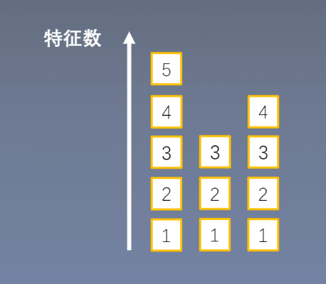
下面代码中,输入数据的形状是 $B \times C \times feature$,(8, 2, 3, 4),表示一个 mini-batch 有 8 个样本,每个样本有 2 个特征,每个特征的维度是 $3 \times 4$。那么就会计算 8 个均值和方差,分别对应每个样本。
1
2
3
4
5
6
7
8
9
10
11
12
13
14
15
16
17
18
19
20
21
batch_size = 8 num_features = 2 features_shape = (3 , 4 )feature_map = torch.ones(features_shape) # 2 Dfeature_maps = torch.stack([feature_map * (i + 1 ) for i in range(num_features)], dim=0 ) # 3 Dfeature_maps_bs = torch.stack([feature_maps for i in range(batch_size)], dim=0 ) # 4 Dln = nn.LayerNorm([2 , 3 , 4 ])output = ln(feature_maps_bs)print ("Layer Normalization" )print (ln.weight.shape)print (feature_maps_bs[0 , ...])print (output[0 , ...])
1
2
3
4
5
6
7
8
9
10
11
12
13
14
Layer Normalization2 , 3 , 4 ])[[[1., 1., 1., 1.], [1., 1., 1., 1.], [1., 1., 1., 1.]] ,[[2., 2., 2., 2.], [2., 2., 2., 2.], [2., 2., 2., 2.]] ])[[[-1.0000, -1.0000, -1.0000, -1.0000], [-1.0000, -1.0000, -1.0000, -1.0000], [-1.0000, -1.0000, -1.0000, -1.0000]] ,[[ 1.0000, 1.0000, 1.0000, 1.0000], [ 1.0000, 1.0000, 1.0000, 1.0000], [ 1.0000, 1.0000, 1.0000, 1.0000]] ], grad_fn=<SelectBackward>)
Layer Normalization 可以设置 normalized_shape 为 (3, 4) 或者 (4)。
Instance Normalization 提出的原因:Batch Normalization 不适用于图像生成。因为在一个 mini-batch 中的图像有不同的风格,不能把这个 batch 里的数据都看作是同一类取标准化。
思路:逐个 instance 的 channel 计算均值和方差。也就是每个 feature map 计算一个均值和方差。
包括 InstanceNorm1d、InstanceNorm2d、InstanceNorm3d。
以InstanceNorm1d为例,定义如下:
1 torch.nn.InstanceNorm1d(num_features, eps =1e-05, momentum =0.1, affine =False , track_running_stats =False )
参数:
num_features:一个样本的特征数,这个参数最重要
eps:分母修正项
momentum:指数加权平均估计当前的的均值和方差
affine:是否需要 affine transform
track_running_stats:True 为训练状态,此时均值和方差会根据每个 mini-batch 改变。False 为测试状态,此时均值和方差会固定
下面代码中,输入数据的形状是 $B \times C \times 2D_feature$,(3, 3, 2, 2),表示一个 mini-batch 有 3 个样本,每个样本有 3 个特征,每个特征的维度是 $2 \times 2 $。那么就会计算 $3 \times 3 $ 个均值和方差,分别对应每个样本的每个特征。如下图所示:
1
2
3
4
5
6
7
8
9
10
11
12
13
14
15
16
17
18
19
batch_size = 3 num_features = 3 momentum = 0.3 features_shape = (2 , 2 )feature_map = torch.ones(features_shape) feature_maps = torch.stack([feature_map * (i + 1 ) for i in range(num_features)], dim=0) feature_maps_bs = torch.stack([feature_maps for i in range(batch_size)], dim=0) "Instance Normalization" )"input data:\n{} shape is {}" .format(feature_maps_bs, feature_maps_bs.shape))instance_n = nn.InstanceNorm2d(num_features=num_features, momentum=momentum) in range(1 ):outputs = instance_n(feature_maps_bs)
输出如下:
1
2
3
4
5
6
7
8
9
10
11
12
13
14
15
16
17
18
19
20
21
22
23
24
25
26
27
28
29
30
31
32
33
34
35
36
37
38
Instance Normalizationis torch.Size()
Group Normalization 提出的原因:在小 batch 的样本中,Batch Normalization 估计的值不准。一般用在很大的模型中,这时 batch size 就很小。
思路:数据不够,通道来凑。 每个样本的特征分为几组,每组特征分别计算均值和方差。可以看作是 Layer Normalization 的基础上添加了特征分组。
注意事项:
不再有 running_mean 和 running_var
$\gamma$ 和 $\beta$ 为逐通道的
定义如下:
1 torch.nn.GroupNorm(num_groups , num_channels , eps =1e-05, affine =True)
参数:
num_groups:特征的分组数量
num_channels:特征数,通道数。注意 num_channels 要可以整除 num_groups
eps:分母修正项
affine:是否需要 affine transform
下面代码中,输入数据的形状是 $B \times C \times 2D_feature$,(2, 4, 3, 3),表示一个 mini-batch 有 2 个样本,每个样本有 4 个特征,每个特征的维度是 $3 \times 3 $。num_groups 设置为 2,那么就会计算 $2 \times (4 \div 2) $ 个均值和方差,分别对应每个样本的每个特征。
1
2
3
4
5
6
7
8
9
10
11
12
13
14
15
batch_size = 2 num_features = 4 num_groups = 2 features_shape = (2 , 2 )feature_map = torch.ones(features_shape) feature_maps = torch.stack([feature_map * (i + 1 ) for i in range(num_features)], dim=0) feature_maps_bs = torch.stack([feature_maps * (i + 1 ) for i in range(batch_size)], dim=0) gn = nn.GroupNorm(num_groups, num_features)outputs = gn(feature_maps_bs)"Group Normalization" )0 ])
输出如下:
1
2
3
4
5
6
7
8
9
10
Group Normalization4 ])[[[-1.0000, -1.0000], [-1.0000, -1.0000]] ,[[ 1.0000, 1.0000], [ 1.0000, 1.0000]] ,[[-1.0000, -1.0000], [-1.0000, -1.0000]] ,[[ 1.0000, 1.0000], [ 1.0000, 1.0000]] ], grad_fn=<SelectBackward>)
 ,Batch Normalization 的可学习参数是$\gamma, \beta$,步骤如下: